Module 17 1-Sample Z-Test
A foundation for making statistical inferences was provided in Modules 11-16. Most of the material in Modules 13 and 15 is related to a 1-Sample Z-test, which is formalized in this module. Other specific hypothesis tests are in Modules 18-21.
17.1 11-Steps of Hypothesis Testing
Hypothesis testing is a rigorous and formal procedure for making inferences about a parameter from a statistic. The 11 steps listed below will help make sure that all aspects important to hypothesis testing are completed. These steps should be used for all hypothesis tests in this and ensuing modules.
- State the rejection criterion (α).
- State the null and alternative hypotheses to be tested and define the parameter(s).
- Identify (and explain why!) the hypothesis test to use (e.g., 1-Sample t, 2-sample t, etc.).
- Collect the data (address study type and if randomization occurred).
- Check all necessary assumptions (describe how you tested the validity).
- Calculate the appropriate statistic(s).
- Calculate the appropriate test statistic.
- Calculate the p-value.
- State your rejection decision about H0.
- Summarize your findings in terms of the problem.
- Compute and interpret an appropriate confidence region for the parameter.
The order of some of these steps is arbitrary. However, Steps 1-3 MUST be completed before collecting data (Step 4). Further note that Step 11 is most important after H0 was rejected to provide a more definitive statement about the value of the parameter (i.e., if the parameter differs from the hypothesized value, then provide a range for which the actual parameter may exist).
17.2 1-Sample Z-Test Specifics
A 1-Sample Z-Test tests H0:μ=μ0, where μ0 represents a specific value of μ, when σ is known. Other specifics of this test were discussed in previous modules and are summarized below.
- Hypothesis: H0:μ=μ0
- Statistic: \(\bar{\text{x}}\)
- Test Statistic: Z=\(\frac{\bar{\text{x}}-\mu_{0}}{\frac{\sigma}{\sqrt{\text{n}}}}\)
- Confidence Region: \(\bar{\text{x}}+\text{Z}^{*}\frac{\sigma}{\sqrt{\text{n}}}\)
- Assumptions:
- σ is known
- n≥30, n≥15 and the population is not strongly skewed, OR the population is normally distributed.
- Use with: Quantitative response, one group (or population), σ known.
The only test that can possibly be confused with a 1-Sample Z-Test is a 1-Sample t-Test (Module 18), which tests the same null hypothesis but when σ is unknown.
17.3 Examples
17.3.1 Intra-class Travel
Below are the 11-steps (Section 17.1) for completing a full hypothesis test for the following situation:
A dean wants to determine if it takes more than 10 minutes, on average, to go between classes. To test this hypothesis, she collected a random sample of 100 intra-class travel times and found a mean of 10.12 mins. Assume from previous studies that the distribution of intra-class times is symmetric with a standard deviation of 1.60 mins. Test the dean’s hypothesis with α=0.10.
- α=0.10.
- H0:μ=10 mins vs. HA:μ>10 mins, where μ is the mean time for ALL intra-class travel events.
- A 1-Sample Z-Test is required because …
- a quantitative variable (intra-class travel time) was measured,
- individuals from one group (or population) is considered (students at the Dean’s school), and
- σ is thought to be known (=1.60 mins).
- The data appear to be part of an observational study (the dean did not impart any conditions on the students) with a random selection of individuals.
- The assumptions are met because …
- n=100≥30, and
- σ is thought to be known (=1.60 mins).
- \(\bar{\text{x}}\)=10.12.
- Z=\(\frac{10.12-10}{\frac{1.60}{\sqrt{100}}}\)=\(\frac{0.12}{0.16}\)=0.75.
- p-value=0.2266.
- H0 is not rejected because the p-value>α=0.10.
- It appears that the mean time for all intra-class travel events is not more than 10 minutes.
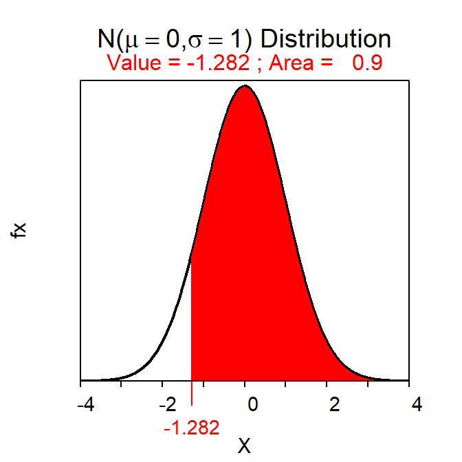
- A 90% lower confidence bound will use Z*=-1.282. The lower confidence bound is thus 10.12-1.282×\(\frac{1.60}{\sqrt{100}}\)=9.91. Thus, I am 90% confident that the mean intra-class travel time is more than 9.91 minutes; further evidence that the mean intra-class travel time is not greater than 10 minutes.
R Appendix:
( z <- distrib(10.12,mean=10,sd=1.60/sqrt(100),lower.tail=FALSE) ) #p-value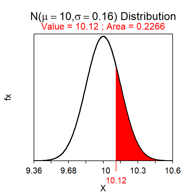
( zstar <- distrib(0.90,lower.tail=FALSE,type="q") ) #z-star