Module 13 Hypothesis Testing - Introduction
A statistic is an imperfect estimate of a parameter because of sampling variability. There are two calculations that use the results of a single sample that recognize this imperfection and allow conclusions to be made about a parameter. First, a researcher may form an a priori hypothesis about a parameter and then use the information in the sample to make a judgment about the “correctness” of that hypothesis. Second, a researcher may use the information in the sample to calculate a range of values that is likely to contain the parameter. The first method is called hypothesis testing and is the subject of this and the next modules. The second method consists of constructing a confidence region, which is introduced in Modules 15 and 16. Specific applications of these two techniques are described in Modules 17-21.
13.1 Hypothesis Testing & The Scientific Method
In its simplest form, the scientific method has four steps:
- Observe and describe a natural phenomenon.
- Formulate a hypothesis to explain the phenomenon.
- Use the hypothesis to predict new observations.
- Experimentally test the predictions.
- Draw a conclusion (from how the observations match the predictions).
If the results of the experiment do not match the predictions, then the hypothesis is rejected and an alternative hypothesis is proposed. If the results of the experiment closely match the predictions, then belief in the hypothesis is gained, though the hypothesis will likely be subjected to further experimentation.
Statistical hypothesis testing is key to using the scientific method in many fields of study and, in fact, closely follows the scientific method in concept. Statistical hypothesis testing begins by formulating two competing statistical hypotheses from a research hypothesis. One of these hypotheses (the null) is used to predict the parameter of interest. Data is then collected and statistical methods are used to determine whether the observed statistic closely matches the prediction made from the null hypothesis or not. Probability (Module 12) is used to measure the degree of matching, with sampling variability taken into account. This process and the theory underlying statistical hypothesis testing is explained in this module.
13.2 Statistical Hypotheses
Hypotheses are classified into two types: (1) research hypothesis and (2) statistical hypotheses. A research hypothesis is a “wordy” statement about the question or phenomenon that the researcher is testing. Four example research hypotheses are:
- A medical researcher is concerned that a new medicine may change patients’ mean pulse rate (from the “known” mean pulse rate of 82 bpm for individuals in the study population not using the new medicine).
- A chemist has invented an additive to car batteries that she thinks will extend the current 36 month average life of a battery.
- An engineer wants to determine if a new type of insulation will reduce the average heating costs of a typical house (which are currently $145 per month).
- A researcher is concerned whether, on average, Alzheimer’s caregivers at a particular facility are clinically depressed (as suggested by a mean Beck Depression Inventory (BDI) score greater than 25)
Research hypotheses are converted to statistical hypotheses that are mathematical and more easily subjected to statistical methods. There are two types of statistical hypotheses: the null hypothesis and the alternative hypothesis.
The null hypothesis, abbreviated as H0, is a specific statement of no difference between a parameter and a specific value or between two parameters. The H0 ALWAYS contains an equals sign because it always represents “no difference” (i.e., “equal”).
The alternative hypothesis, abbreviated as HA, always states that there is some sort of difference between a parameter and a specific value or between two parameters. The type of difference comes from the research hypothesis and will require use of a less than (“<”), greater than (“>”), or not equals (≠) sign.
Null and alternative hypotheses that correspond to the four research hypotheses above are:
- HA:μ≠82 and H0:μ=82 (where μ represents the mean pulse rate for individuals in the study population that take the new medicine; thus, the alternative hypothesis represents a change from the “normal” pulse rate).
- HA:μ>36 and H0:μ=36 (where μ represents the mean life of batteries with the new additive; thus, this alternative hypothesis represents an extension of the current battery life).
- HA:μ<145 and H0:μ=145 (where μ represents the mean monthly heating bill for houses that receive the new type of insulation; thus, this alternative hypothesis represents a decline in heating bills from the previous “normal” amount).
- HA:μ>25 and H0:μ=25 (where μ represents the mean BDI score; thus, this alternative hypothesis represents a mean score that indicates clinical depression).
The sign used in the alternative hypothesis comes directly from the wording of the research hypothesis (Table 13.1). An alternative hypothesis that contains the ≠ sign is called a two-tailed alternative, as the parameter can be “not equal” in two ways; i.e., less than or greater than. Alternative hypotheses with the < or the > signs are called one-tailed alternatives.
| < | > | \(\neq\) |
|---|---|---|
| is less than | is greater than | is not equal to |
| is fewer than | is more than | is different from |
| is lower than | is larger than | has changed from |
| is shorter than | is longer than | is not the same as |
| is smaller than | is increased from | |
| is below | is above | |
| is reduced from | is better than | |
| is at most | is at least | |
| is not more than | is not less than |
The null hypothesis is easily constructed from the alternative hypothesis by replacing the sign in the alternative hypothesis with an equals sign.
13.2.1 Hypothesis Testing Concept
Statistical hypothesis testing begins by using the null hypothesis to predict what value one should expect for the mean in a sample. So, for the Square Lake example (from Module 1), if H0:μ=105 and HA:μ<105, then one would expect, if the null hypothesis is true, that the observed sample mean would be 105. If sampling variability did not exist, then one would conclude that the null hypothesis was incorrect if the observed sample mean was NOT equal to 105. In other words, one would conclude that the population mean was not equal to 105.
Of course, sampling variability does exist and it complicates matters. The simple interpretation of not supporting H0 because the observed sample mean did not equal the hypothesized population mean canNOT be made because, with sampling variability, one would not expect a statistic to exactly equal the parameter in the population from which the sample was extracted. For example, even if the null hypothesis was correct, one would not expect, with sampling variability, the observed sample mean to exactly equal 105; rather, one would expect the observed sample mean to be reasonably close to 105.
Thus, hypothesis testing is a process to determine if the difference between the observed statistic and the expected statistic based on the null hypothesis is “large” relative to sampling variability. For example, the standard error of \(\bar{\text{x}}\) for samples of n=50 in the Square Lake example is \(\frac{\sigma}{\sqrt{n}}=\)\(\frac{31.49}{\sqrt{50}}\)=4.45. With this amount of sampling variability, an observed sample mean of 103 would be considered reasonably close to 105 and one would have more belief in H0:μ=105 (Figure 13.1). However, an observed sample mean of 90 is further away from 105 than one would expect based on sampling variability alone and belief in H0:μ=105 would lessen (Figure 13.1).
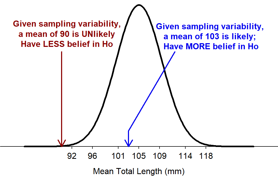
Figure 13.1: Sampling distribution of samples means of n=50 from the Square Lake population ASSUMING that μ=105.
While the above procedure is intuitively appealing, the conclusions are not as clear when the examples chosen (i.e., samples means of 103 and 90) are not as extremely close or distant from the null hypothesized value. For example, what would one conclude if the observed sample mean was 97?.
A first step in creating a more objective decision criteria is to compute the “p-value.” A p-value is the probability of the observed statistic or a value of the statistic more extreme assuming that the null hypothesis is true. The p-value is described in more detail below given its centrality to making conclusions about statistical hypotheses.
The meaning of the phrase “or more extreme” in the p-value definition is derived from the sign in HA (Figure 13.2). If HA is the “less than” situation, then “or more extreme” means “shade to the left” for the probability calculation. The “greater than” situation is defined similarly but would result in shading to the “right.” In the “not equals” situation, “or more extreme” means further into the tail AND the exact same size of tail on the other side of the distribution. It is clear from Figure 13.2 why “less than” and “greater than” are called one-tailed alternatives and “not equals” is called a two-tailed alternative.
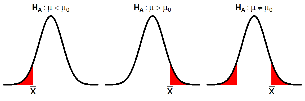
Figure 13.2: Depiction of “or more extreme” (red areas) in p-values for the three possible alternative hypotheses.
The “assuming that the null hypothesis is true” phrase is used to define a μ for the sampling distribution on which the p-value will be calculated. This sampling distribution is called the null distribution because it depends on the value of μ from the null hypothesis. One must remember that the null distribution represents the distribution of all possible sample means assuming that the null hypothesis is true; it does NOT represent the actual sample means.58 The null distribution in the Square Lake example is thus \(\bar{\text{x}}\)~N(105,4.45) because n=50≥30 (so the Central Limit Theorem holds), H0:μ=105, and SE=\(\frac{31.49}{\sqrt{50}}\)=4.45.
The p-value is computed with a “forward” normal distribution calculation on the null sampling distribution. For example, suppose that a sample mean of 100 was observed with n=50 from Square Lake (as it was in Table 2.2). The p-value in this case would be “the probability of observing \(\bar{\text{x}}\)=100 or a smaller value assuming that μ=105.” This probability is computed by finding the area to the left of 100 on a N(105,4.45) null distribution and is the exact same type of calculation as that made in Section 12.2. Thus, this p-value of p=0.1308 is computed as below and shown in Figure 13.3.
( distrib(100,mean=105,sd=31.49/sqrt(50)) )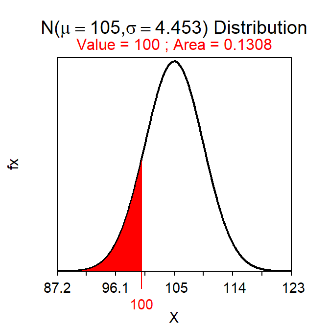
Figure 13.3: Depiction of the p-value for the Square Lake example where \(\bar{\text{x}}\)=100 and HA:μ<105.
Interpreting the p-value requires critically thinking about the p-value definition and how it is calculated. Small p-values appear when the observed statistic is “far” from the null hypothesized value. In this case there is a small probability of seeing the observed statistic ASSUMING that H0 is true. Thus, the assumption is likely wrong and H0 is likely incorrect. In contrast, large p-values appear when the observed statistic is close to the null hypothesized value suggesting that the assumption about H0 may be correct.
The p-value serves as a numerical measure on which to base a conclusion about H0. To do this objectively requires an objective definition of what it means to be a “small” or “large” p-value. Statisticians use a cut-off value, called the rejection criterion and symbolized with α, such that p-values less than α are considered small and would result in rejecting H0 as a viable hypothesis. The value of α is typically small, usually set at 0.05, although α=0.01 and α=0.10 are also commonly used.
The choice of α is made by the person conducting the hypothesis test and is based on how much evidence a researcher demands before rejecting H0. Smaller values of α require a larger difference between the observed statistic and the null hypothesized value and, thus, require “more evidence” of a difference for the H0 to be rejected. For example, if rejection of the null hypothesis will be heavily scrutinized by regulatory agencies, then the researcher may want to be very sure before claiming a difference and should then set α at a smaller value, say α=0.01. The actual choice for α MUST be made before collecting any data and canNOT be changed once the data has been collected. In other words, once the data are in hand, a researcher cannot lower or raise α to achieve a desired outcome regarding H0.
The value of the rejection criterion (α) is set by the researcher BEFORE data is collected.
The null hypothesis in the Square Lake example is not rejected because the p-value (i.e., 0.1308) is larger than any of the common values of α. Thus, the conclusion in this example is that it is possible that the mean of the entire population is equal to 105 and it is not likely that the population mean is less than 105. In other words, observing a sample mean of 100 is likely to happen based on random sampling variability alone and it is unlikely that the null hypothesized value is incorrect.
13.3 Example p-value Calculations
The following are examples for calculating a p-value given typical information. I suggest that you following these steps when calculating a p-value
- Identify H0 and HA
- Define the p-value specific to the situation.
- In the generic p-value definition (“probability of the observed statistic or a value more extreme assuming the H0 is true) replace”observed statistic” with the value of \(\bar{\text{x}}\), “more extreme” with “less,” “greater,” or “different” depending on HA, and “the H0 is true” with the specific value of μ in H0.
- Draw the null distribution.
- This is the sampling distribution assuming that H0 is true. Thus, it will be centered on the μ in H0 and will use a standard error of \(\frac{\sigma}{\sqrt{\text{n}}}\).
- Compute the p-value.
- This will be a FORWARD calculation on a normal distribution centered on μ from H0 with an area shaded “more extreme” (depending on HA) of \(\bar{\text{x}}\).
- If HA is a “not equals” then “more extreme” means into the nearest tail and then multiplied by 2.
- Make a decision about H0. If the question has a context then the parameter should be stated within the context of the question.
- If the p-value<α then reject H0 (in favor of HA.
- If the p-value>α then do not reject (DNR) H0 (in favor of HA).
Example - Taking a Quiz (Less Than HA)
Suppose that I hypothesized that the mean time to take a quiz is less than 100 minutes. Further suppose that, in a sample of 30 students, the mean time to take the quiz was 95.2 minutes and that σ=20 and α=0.10.
- H0: μ=100 versus HA: μ<100, where μ is the mean time to take a quiz.
- The p-value is the “probability that \(\bar{\text{x}}\)=95.2 or less assuming that μ=100.”
- The null distribution will have a mean of 100 and a SE of \(\frac{20}{\sqrt{30}}\)=3.651. See drawing below.
- The p-value is 0.0943 as computed below.
- Reject H0 because p-value (0.0943) < α (0.10). Thus, it appears that the MEAN time for ALL students to take the quiz is less than 100 minutes.
distrib(95.2,mean=100,sd=20/sqrt(30))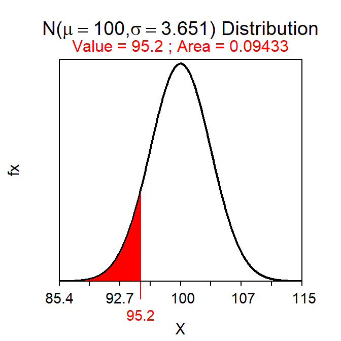
Example - Walking to Class (Greater Than HA)
Suppose that I hypothesized that the mean time to walk between the Science Center and the Ponzio Center is more than 7 minutes. Further suppose that, in a sample of 50 students, the mean time to make this walk was 8.3 minutes and that σ=1.3 and α=0.05.
- H0: μ=7 versus HA: μ>7, where μ is the mean time to walk between the Science Center and the Ponzio Center.
- The p-value is the “probability that \(\bar{\text{x}}\)=8.3 or greater assuming that μ=7.”
- The null distribution will have a mean of 7 and a SE of \(\frac{1.3}{\sqrt{50}}\)=0.184. See drawing below.
- The p-value is 0.0000000000007687 as computed below. Note that the p-value does not need all of these decimals and, thus, I will usually show this as <0.00005.
- Reject H0 because p-value < α (0.05). Thus, it appears that the MEAN time for ALL students to walk between the Science Center and the Ponzio Center is greater than 7 minutes.
distrib(8.3,mean=7,sd=1.3/sqrt(50),lower.tail=FALSE)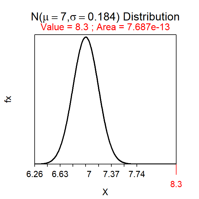
Exapmle Preparation Guide Time (Not Equals HA)
Suppose that I hypothesized that the mean time students spend preparing the preparation guide is different than 30 minutes and that, in a sample of 40 students, the mean preparation time was 33.8 minutes. Further, suppose that σ=9.7 and α=0.01.
- H0: μ=30 versus HA: μ≠30, where μ is the mean time preparing for the prep check.
- The p-value is the “probability that \(\bar{\text{x}}\)=33.8 or no assuming that μ=30.”
- The null distribution will have a mean of 30 and a SE of \(\frac{9.7}{\sqrt{40}}\)=1.534. See drawing below.
- The half p-value is 0.0066 as computed below. Thus, the p-value is 0.0132
- Do not reject H0 because p-value (0.0132) > α (0.01). Thus, it appears that the MEAN time that ALL students spend preparing for the prep check is not different than 30 minutes.
distrib(33.8,mean=30,sd=9.7/sqrt(40),lower.tail=FALSE)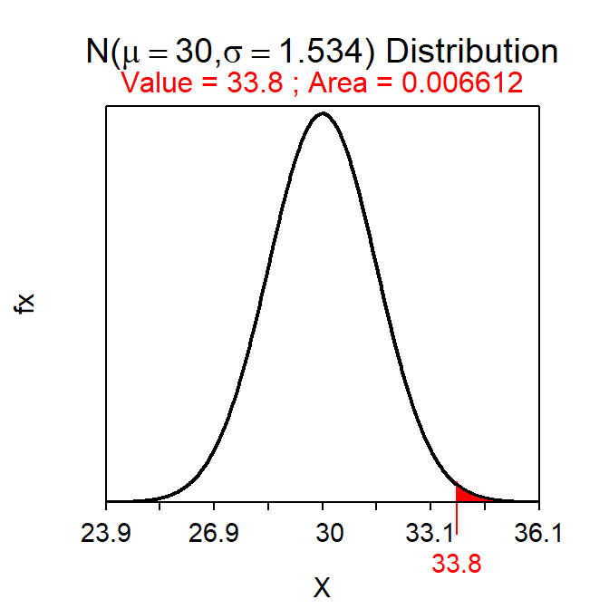
When HA is a “not equals” then the area shaded on the null distribution is into the nearest tail. In this case, because \(\bar{\text{x}}\) (=33.8) was greater than the mean of the distribution (=30), I shaded to the right (into the nearer “upper tail”). If the \(\bar{\text{x}}\) had been lower, I would have shaded to the left. In these situations (i.e., when HA is a “not equals”) then the area returned by distrib() must be multiplied by two to get the p-value (to account for both tails of the same size).
13.4 Hypothesis Testing Concept Summary
In summary, hypotheses are statistically examined with the following procedure.
- Construct null and alternative hypotheses from the research hypothesis.
- Construct an expected value of the statistic based on the null hypothesis (i.e., assume that the null hypothesis is true).
- Calculate an observed statistic from the individuals in a sample.
- Compare the difference between the observed statistic and the expected statistic based on the null hypothesis in relation to sampling variability (i.e., calculate a test statistic and p-value).
- Use the p-value to determine if this difference is “large” or not.
- If this difference is “large” (i.e., p-value<α), then reject the null hypothesis.
- If this difference is not “large” (i.e., p-value>α), then “Do Not Reject” the null hypothesis.
Statisticians say “do not reject H0” rather than “accept H0 as true” when the p-value >α for two reasons. First, there are several other possible values, besides the specific value in the null hypothesis, that would lead to “do not reject” conclusions. For example, if a null hypothesized value of 105 was not rejected, then values of 104.99, 104.98, etc. would also likely not be rejected.59 So, we don’t say that we “accept” a particular hypothesized value when we know many other values would also be “accepted.”
Second, the null hypothesis is almost always not true. Consider the null hypothesis of the Square Lake example (i.e., “that the mean length is 105 mm”). The mean length of fish in Square Lake is undoubtedly not exactly equal to 105. It may be 104.9, 105.01, or some other more disparate value. The point is that the specific value of the hypothesis is likely never true, especially for a continuous variable. The problem is that it takes large amounts of data to be able to distinguish means that are very close to the true population mean (i.e., it is difficult to distinguish between 104.9 and 105 when sampling variability is present). Very often we will not take a sample size large enough to distinguish these subtle differences. Thus, we will say that we “do not reject H0” because there simply was not enough data to reject it.