Module 3 Data Production
Statistical inference is the process of making conclusions about a population from the results of a single sample. To make conclusions about the larger population, the sample must fairly represent the larger population. Thus, the proper collection (or production) of data is critical to statistics (and science in general). In this module, two ways of producing data – (1) Experiments and (2) Observational Studies – are described.
Inferences cannot be made if data are not properly collected.
3.1 Experiments
An experiment deliberately imposes a condition on individuals to observe the effect on the response variable. In a properly designed experiment, all variables that are not of interest are held constant, whereas the variable(s) that is (are) of interest are changed among treatments. As long as the experiment is designed properly (see below), differences among treatments are either due to the variable(s) that were deliberately changed or randomness (chance). Methods to determine if differences were likely due to randomness are developed in later modules. Because we can determine if differences most likely occurred due too randomness or changes in the variables, strong cause-and-effect conclusions can be made from data collected from carefully designed experiments.
3.1.1 Single-factor Experiments
A factor is a variable that is deliberately manipulated to determine its effect on the response variable. A factor is sometimes called an explanatory variable because we are attempting to determine how it affects (or “explains”) the response variable. The simplest experiment is a single-factor experiment where the individuals are split into groups defined by the categories of a single factor.
For example, suppose that a researcher wants to examine the effect of temperature on the total number of bacterial cells after two weeks. They have inoculated 120 agars13 with the bacteria and placed them in a chamber where all environmental conditions (e.g., temperature, humidity, light) are controlled exactly. The researchers will use only two temperatures in this simple experiment – 10oC and 15oC. All other variables are maintained at constant levels. Thus, temperature is the only factor in this simple experiment because it is the only variable manipulated to different values to determine its impact on the number of bacterial cells.
In a single-factor experiment only one explanatory variable (i.e., factor) is allowed to vary; all other explanatory variables are held constant.
Levels are the number of categories of the factor variable. In this example, there are two levels – 10oC and 15oC. Treatments are the number of unique conditions that individuals in the experiment are exposed to. In a single-factor experiment, the number of treatments is the same as the number of levels of the single factor. Thus, in this simple experiment, there are two treatments – 10oC and 15oC. Treatments are discussed more thoroughly in the next section.
The number of replicates in an experiment is the number of individuals that will receive each treatment. In this example, a replicate is an inoculated agar. The number of replicates is the number of inoculated agars that will receive each of the two temperature treatments. The number of replicates is determined by dividing the total number of available individuals (120) by the number of treatments (2). Thus, in this example, the number of replicates is 60 (=\(\frac{120}{2}\)) inoculated agars.
The agars used in this experiment will be randomly allocated to the two temperature treatments. All other variables – humidity, light, etc. – are kept the same for each treatment. At the end of two weeks, the total number of bacterial cells on each agar (i.e., the response variable) will be recorded and compared between the agars kept at both temperatures.14 Any difference in mean number of bacterial cells will be due to either different temperature treatments or randomness, because all other variables were the same between the two treatments.
Differences among treatments are either caused by randomness (chance) or the factor.
The single factor is not restricted to just two levels. For example, more than two temperatures, say 10oC, 12.5oC, 15oC, and 17.5oC, could have been tested. With this modification, there is still only one factor – temperature – but there are now four levels (and four treatments).
3.1.2 Multi-factor Experiments – Design and Definitions
More than one factor can be tested in an experiment. In fact, it is more efficient to have a properly designed experiment where more than one factor is varied at a time than it is to use separate experiments in which only one factor is varied in each. However, before showing this benefit, let’s examine the definitions from the previous section in a multi-factor experiment.
Suppose that the previous experiment was modified to also examine the effect of relative humidity on the number of bacteria cells. This modified experiment has two factors – temperature and relative humidity. In this case, we would say that there are two levels of temperature (10oC or 15oC) and four levels of relative humidity (20%, 40%, 60%, and 80%). In other words, keep the levels separate so that you have a number of levels for each factor.
You should list as many numbers of levels as you have factors in the experiment.
The number of treatments, or combinations of all factors, in this experiment is found by multiplying the levels of all factors (i.e., 2×4=8 in this case). The number of replicates in this experiment is now 15 (=\(\frac{120}{8}\); total number of available agars divided by the number of treatments).
The number of treatments is determined for the overall experiment, whereas the number of levels is determined for each factor.
A drawing of the experimental design can be instructive (Table 3.1). The drawing is a table where the levels of one factor are shown in the rows of the first column and the levels of the other factor are shown in the rows of the second column such that each level of the first factor is matched with one of the levels of the second factor. With this, the number of rows in the table is the number of treatments in the experiment. I also like to include a column that shows the number of replicates in each treatment and the individuals randomly allocated to each treatment.15
| Temp. | Rel. Hum. | # Reps | Agars |
|---|---|---|---|
| 10oC | 20% | 15 | 79, 78, 14, 63, 41, 115, 107, 59, 35, 110, 8, 46, 64, 99, 37 |
| 10oC | 40% | 15 | 38, 81, 48, 74, 36, 77, 95, 65, 91, 26, 98, 1, 97, 108, 62 |
| 10oC | 60% | 15 | 39, 42, 82, 47, 101, 106, 29, 113, 2, 53, 18, 32, 52, 34, 117 |
| 10oC | 80% | 15 | 100, 43, 75, 116, 67, 54, 10, 102, 16, 92, 88, 40, 17, 96, 33 |
| 15oC | 20% | 15 | 87, 70, 13, 111, 89, 85, 80, 83, 112, 86, 6, 19, 21, 84, 93 |
| 15oC | 40% | 15 | 12, 45, 66, 31, 30, 22, 90, 72, 7, 120, 27, 50, 23, 71, 69 |
| 15oC | 60% | 15 | 25, 103, 109, 94, 15, 55, 58, 61, 60, 56, 11, 57, 73, 44, 119 |
| 15oC | 80% | 15 | 104, 68, 20, 51, 24, 5, 114, 4, 28, 118, 105, 76, 9, 3, 49 |
3.1.3 Multi-factor Experiments – Benefits
The analysis of a multi-factor experimental design is more involved than what will be shown in this course. However, multi-factor experiments have many benefits, which can be illustrated by comparing a multi-factor experiment to separate single-factor experiments. For example, consider separate single-factor experiments to separately determine the effect of temperature and relative humidity on bacterial growth (further assume that the agars can be used in only one of these separate experiments).
To conduct these two separate experiments, the 120 available agars are randomly split into two equally-sized groups of 60. The first 60 will then be split into two groups of 30 for the first experiment with two temperatures. The second 60 will then be split into four groups of 15 for the second experiment with four relative humidities. These separate single-factor experiments are summarized in Table 3.2.
| Temp. | # Reps | Agars |
|---|---|---|
| 10oC | 30 | 79, 78, 14, 63, 41, 115, 107, 59, 35, 110 , … |
| 15oC | 30 | 39, 42, 82, 47, 101, 106, 29, 113, 2, 53 , … |
| Rel. Hum. | # Reps | Agars |
|---|---|---|
| 20% | 15 | 87, 70, 13, 111, 89, 85, 80, 83, 112, 86, 6, 19, 21, 84, 93 |
| 40% | 15 | 12, 45, 66, 31, 30, 22, 90, 72, 7, 120, 27, 50, 23, 71, 69 |
| 60% | 15 | 25, 103, 109, 94, 15, 55, 58, 61, 60, 56, 11, 57, 73, 44, 119 |
| 80% | 15 | 104, 68, 20, 51, 24, 5, 114, 4, 28, 118, 105, 76, 9, 3, 49 |
The key to examining the benefits of the multi-factor experiment is to determine the number of individuals that give “information” about (i.e., are exposed to) each factor. In the two-factor experiment all 120 individuals were exposed to one of the temperature levels with 60 individuals exposed to each level (Table 3.1). In contrast, only 30 individuals were exposed to these levels in the single-factor experiment (Table 3.2-Top). In addition, in the two-factor experiment all 120 individuals were exposed to one of the relative humidity levels with 30 individuals exposed to each level (Table 3.1). Again, this is in contrast to the single-factor experiment where only 15 individuals were exposed to each of these levels (Table 3.2-Bottom). Thus, the first advantage of multi-factor experiments is that the available individuals are used more efficiently. In other words, more “information” (i.e., the responses of more individuals) is obtained from a multi-factor experiment than from combinations of single-factor experiments.16
A properly designed multi-factor experiment also allows researchers to determine if multiple factors interact to impact an individual’s response. For example, consider the hypothetical results from this experiment in Figure 3.1-Left.17 The effect of relative humidity is to increase the growth rate for those individuals at 10oC but to decrease the growth rate for those individuals at 15oC. That is, the effect of relative humidity differs depending on the level of temperature. When the effect of one factor differs depending on the level of the other factor, then the two factors are said to interact. Interactions cannot be determined from the two single-factor experiments because the same individuals are not exposed to levels of the two factors at the same time.
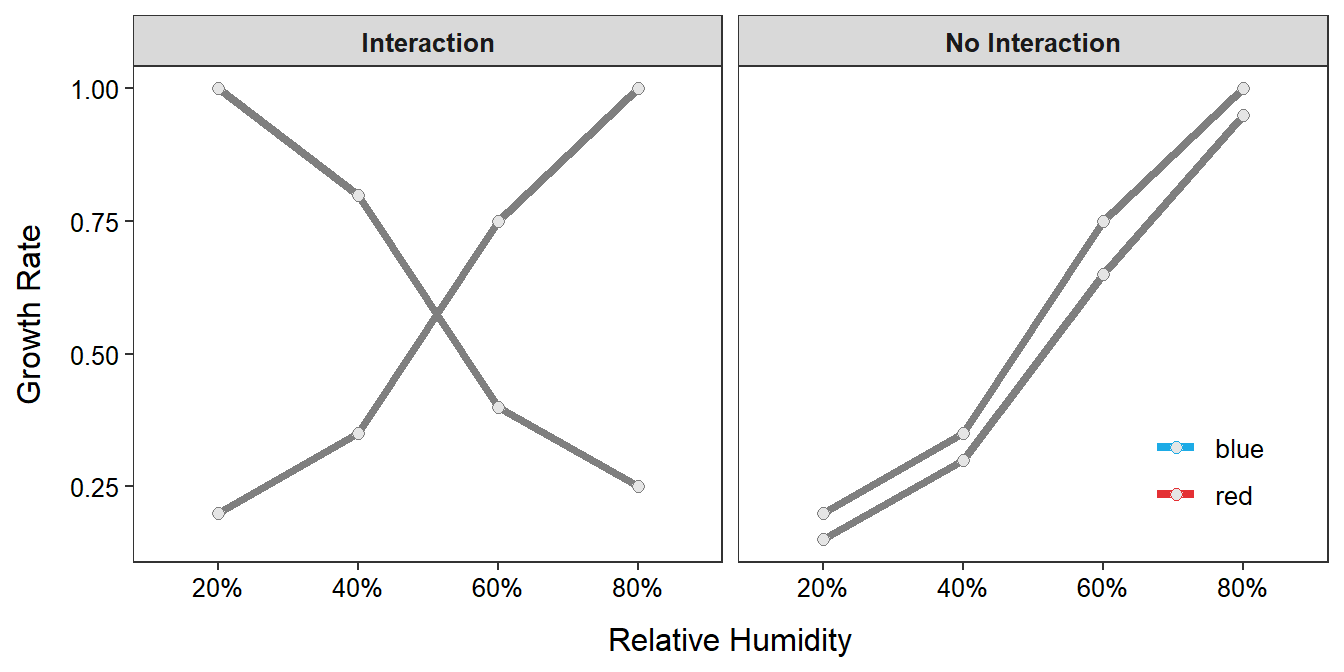
Figure 3.1: Mean growth rates in a two-factor experiment that depict an interaction effect (left) and no interaction effect (right).
Multi-factor experiments are used to detect the presence or absence of interaction, not just the presence of it. The hypothetical results in Figure 3.1-Right show that the growth rate increases with increasing relative humidity at about the same rate for both temperatures. Thus, because the effect of relative humidity is the same for each temperature (and vice versa), there does not appear to be an interaction between the two factors. Again, this could not be determined from the separate single-factor experiments.
3.1.4 Allocating Individuals
Individuals18 should be randomly allocated (i.e., placed into) to treatments. Randomization will tend to even out differences among groups for variables not considered in the experiment. In other words, randomization should help assure that all groups are similar before the treatments are imposed. Thus, randomly allocating individuals to treatments removes any bias (foreseen or unforeseen) from entering the experiment.
In the single-factor experiment above – two treatments of temperature – there were 120 agars. To randomly allocate these individuals to the treatments, 60 pieces of paper marked with “10” and 60 marked with “15” could be placed into a hat. One piece of paper would be drawn for each agar and the agar would receive the temperature found on the piece of paper. Alternatively, each agar could be assigned a unique number between 1 and 120 and pieces of paper with these numbers could be placed into the hat. Agars corresponding to the first 60 numbers drawn from the hat could then be placed into the first treatment. Agars for the next (or remaining) 60 numbers would be placed in the second treatment. This process is essentially the same as randomly ordering 120 numbers.
A random order of numbers is obtained with R by including the count of numbers as the only argument to sample(). For example, randomly ordering 1 through 120 is accomplished with19
sample(120)#R> [1] 79 78 14 63 41 115 107 59 35 110 8 46 64 99 37 38 81 48
#R> [19] 74 36 77 95 65 91 26 98 1 97 108 62 39 42 82 47 101 106
#R> [37] 29 113 2 53 18 32 52 34 117 100 43 75 116 67 54 10 102 16
#R> [55] 92 88 40 17 96 33 87 70 13 111 89 85 80 83 112 86 6 19
#R> [73] 21 84 93 12 45 66 31 30 22 90 72 7 120 27 50 23 71 69
#R> [91] 25 103 109 94 15 55 58 61 60 56 11 57 73 44 119 104 68 20
#R> [109] 51 24 5 114 4 28 118 105 76 9 3 49Thus, the first five (of 60) agars in the 10oC treatment are 79, 78, 14, 63, and 41 (Table 3.2-Top). The first five (of 60) agars in the 15oC treatment are 87, 70, 13, 111, and 89 (Table 3.2-Top). In the modified experiment with two factors – temperature and relative humidity – with eight treatments containing 15 agars each, the random numbers would be divided into 8 groups each with 15 numbers. The allocation of individuals was shown in Table 3.1.
Individuals should be randomly allocated to treatments to remove bias.
3.1.5 Design Principles
There are many other methods of designing experiments and allocating individuals that are beyond the scope of this course.20 However, all experimental designs contain the following three basic principles.
- Control the effect of variables on the response variable by deliberately manipulating factors to certain levels and maintaining constancy among other variables.
- Randomize the allocation of individuals to treatments to eliminate bias.
- Replicate individuals (use many individuals) in the experiment to reduce chance variation in the results.
Proper control in an experiment allows for strong cause-and-effect conclusions to be made (i.e., to state that an observed difference in the response variable was due to the levels of the factor or chance variation rather than some other foreseen or unforeseen variable). Randomly allocating individuals to treatments removes any bias that may be included in the experiment. For example, if we do not randomly allocate the agars to the treatments, then it is possible that a set of all “poor” agars may end up in one treatment. In this case, any observed differences in the response may not be due to the levels of the factor but to the prior quality of the agars. Replication means that there should be more than one or a few individuals in each treatment. This reduces the effect of each individual on the overall results. For example, if there was one agar in each treatment, then, even with random allocation, the effect of that treatment may be due to some inherent properties of that agar rather than the levels of the factors. Replication, along with randomization, helps assure that the groups of individuals in each treatment are as alike as possible at the start of the experiment.
3.2 Observational Studies – Sampling
In observational studies the researcher has no control over any of the variables observed for an individual. The researcher simply observes individuals, disturbing them as little as possible, trying to get a “picture” of the population. Observational studies cannot be used to make cause-and-effect statements because all variables that may impact the outcome may not have been measured or specifically controlled. Thus, any observed difference among groups may be caused by the variables measured, some other unmeasured variables, or chance (randomness).
Consider the following as an example of the problems that can occur when all variables are not measured. For many years scientists thought that the brains of females weighed less than the brains of males. They used this finding to support all kinds of ideas about sex-based differences in learning ability. However, these earlier researchers failed to measure body weight, which is strongly related to brain weight in both males and females. After controlling for the effect of differences in body weights, there was no difference in brain weights between the sexes. Thus, many sexist ideas persisted for years because cause-and-effect statements were inferred from data where all variables were not considered.
Strong cause-and-effect statements CANNOT be made from observational studies.
In observational studies, it is important to understand to which population inferences will refer.21 To make useful inferences from a sample, the sample must be an unbiased representation of the population. In other words, it must not systematically favor certain individuals or outcomes.
For example, consider that you want to determine the mean length of all fish in a particular lake (e.g., Square Lake from Module 2). Using a net with large mesh, such that only large fish are caught, would produce a biased sample because interest is in all fish not just the large fish. Setting the nets near spawning beds (i.e., only adult fish) would also produce a biased sample. In both instances, a sample would be collected from a population other than the population of interest. Thus it is important to select a sample from the specified population.
It is important to understand the population before considering how to take a sample.
3.2.1 Types of Sampling Designs
Three common types of sampling designs – voluntary response, convenience, and probability-based samples – are considered in this section. Voluntary response and convenience samples tend to produce biased samples, whereas proper probability-based samples will produce an unbiased sample. An unbiased sample is desired as it means that no segment of the population was systematically over- or under-represented in the sample.
A voluntary response sample consists of individuals that have chosen themselves for the sample by responding to a general appeal. An example of a voluntary response sample would be the group of people that respond to a general appeal placed in the school newspaper. If the population of interest in this sample was all students at the school, then this type of general appeal would likely produce a biased sample of students that (i) read the school newspaper, (ii) feel strongly about the topic, or (iii) both. A more obvious example is the group of people that respond to a Facebook, Twitter, or Instagram poll.
A convenience sample consists of individuals who are easiest to reach for the researcher. An example of a convenience sample is when a researcher queries only those students in a particular class. This sample is “convenient” because the individuals are easy to gather. However, if the population of interest was all students at the school, then this type of sample would likely produce a biased sample of students that is likely of (i) one major or another, (ii) one or a few “years-in-school” (e.g., Freshman or Sophomores), or (iii) both.
In probability-based sampling, each individual of the population has a known chance of being selected for the sample. The simplest probability-based sample is the Simple Random Sample (SRS) where each individual has the same chance of being selected. Proper selection of an SRS requires each individual to be assigned a unique number. The SRS is then formed by choosing random numbers and collecting the individuals that correspond to those numbers.
For example, an auditor may need to select a sample of 30 financial transactions from all transactions of a particular bank during the previous month. Because each transaction is numbered, the auditor may know that there were 1112 transactions during the previous month (i.e., the population). The auditor would then number each transaction from 1 to 1112, randomly select 30 numbers (with no repeats) from between 1 and 1112, and then physically locate the 30 transactions that correspond to the 30 selected numbers. Those 30 transactions are the SRS.
Random numbers are selected in R by including the population size as the first and sample size as the second argument to sample(). For example, 30 numbers from between 1 and 1112 is selected with
sample(1112,30)#R> [1] 684 986 155 638 10 390 381 265 474 707 699 97 752 681 565
#R> [16] 739 59 324 861 637 490 911 446 406 846 516 269 1052 384 1105Thus, accounts 684, 986, 155, 638, and 10 would be the first five (of 30) selected.
There are other more complex types of probability-based samples that are beyond the scope of this course.22 However, the goal of these more complex types of samples is generally to impart more control into the sampling design.
A proper SRS requires each individual in the population to be assigned a unique number.
If the population is such that a number cannot be assigned to each individual, then the researcher must try to use a method for which they feel each individual has an equal chance of being selected. Usually this means randomizing the technique rather than the individuals. In the fish example discussed previously, the researcher may consider choosing random mesh sizes, random locations for placing the net, or random times for placing the net. Thus, in many real-life instances, the researcher simply tries to use a method that is likely to produce an SRS or something very close to it.
If a number cannot be assigned to each individual in the population, then the researcher should randomize the “technique” to assure as close to a random sample as possible.
Polls, campaign or otherwise, are examples of observational studies that you are probably familiar with. The following are links where various aspects of polling are discussed.
3.2.2 Of What Value are Observational Studies?
Properly designed experiments can lead to “cause-and-effect” statements, whereas observational studies (even properly designed) are unlikely to lead to such statements. Furthermore, in the last section, it was suggested that it is very difficult to take a proper probability-based sample because it is hard to assign a number to each individual in the population (precisely because entire populations are very difficult to “see”). So, do observational studies have any value? There are at least three reasons why observational studies are useful.
The scientific method begins with making an observation about a natural phenomenon. Observational studies may serve to provide such an observation. Alternatively, observational studies may be deployed after an observation has been made to see if that observation is “prevalent” and worthy of further investigation. Thus, observational studies may lead directly to hypotheses that form the basis of experiments.
Experiments are often conducted under very confined and controlled conditions so that the effect of one or more factors on the response variable can be identified. However, at the conclusion of an experiment it is often questioned whether a similar response would be observed “in nature” under much less controlled conditions. For example, one might determine that a certain fertilizer increases growth of a certain plant in the greenhouse, with consistent soil characteristics, temperatures, lighting, etc. However, it is a much different, and, perhaps, more interesting, question to determine if that fertilizer elicits the same response when applied to an actual field. This follow-up question would require an observational study.
Finally, there are situations where conducting an experiment simply cannot be done, either for ethical, financial, size, or other constraints. For example, it is generally accepted that smoking causes cancer in humans even though an experiment where one group of people was forced to smoke while another was not allowed to smoke has not been conducted. Similarly, it is also very difficult to perform valid experiments on “ecosystems.” In these situations, an observational study is simply the best study allowable. Cause-and-effect statements are arrived at in these situations because observational studies can be conducted with some, though not absolute, control and control can be imparted mathematically into some analyses.23 In addition, a “preponderance of evidence” may be arrived at if enough observational studies point to the same conclusion.
An agar, in this case, is a petri dish with a growth medium for the bacteria.↩︎
How to randomly allocate individuals to treatments is shown in Section 3.1.4.↩︎
The real importance of this advantage will become apparent when statistical power is introduced in Module 13.↩︎
The means of each treatment are plotted and connected with lines in this plot.↩︎
When discussing experiments, an “individual” is often referred to as a “replicate” or an “experimental unit.”↩︎
In the results below the 120 numbers must be wrapped because they will not fit the page from left-to-right. The numbers is the square brackets at the beginning of each line are NOT random numbers, but are the POSITION of the first number on that line. Thus, the “74” shown on the second line is the 19th random number and the “51” shown on the last line is the 109th random number.↩︎
Other common designs include blocked, Latin square, and nested designs.↩︎
Thus, it is very important to first perform an IVPPS as discussed in Module 2.↩︎
For example, stratified samples, nested, and multistage samples.↩︎
These analyses are beyond the scope of this book, though.↩︎