Module 7 Normal Distribution Calculations
The normal distribution was introduced in Module 6 and the 68-95-99.7% Rule was used to find the percentage of individuals with particular values of the variable (i.e., a forward calculation) or to find the value or values of the variable with a certain percentage of individuals (i.e., a reverse calculation). Unfortunately, the 68-95-99.7% Rule can only be used if the value (or values) in the question fall exactly 1, 2, or 3 standard deviations away from the mean. In other words, questions relative to non-integer numbers of standard deviations away from the mean can not be found with the 68-95-99.7% Rule and will require special tables or computer software.
In this course, we will use a function from the NCStats package in R to perform these calculations. How you use this function depends on whether it is a forward or reverse calculation (see Section 6.5).
7.1 Forward Calculations
The area under a normal curve relative to a particular value is computed in R with distrib(), with the particular value as the first argument and the mean (μ) and standard deviation (σ) of the normal distribution in the mean= and sd= arguments, respectively. The distrib() function defaults to finding the area to the left of the particular value; it can find the area to the right of the particular value by including lower.tail=FALSE.
For example, suppose that the heights of a population of students is known to be H~N(66,3). The proportion of students in this population that have a height less than 71 inches is with
( distrib(71,mean=66,sd=3) )which produces Figure 7.1. Thus, approximately 95.2% of students in this population have a height less than 71 inches.
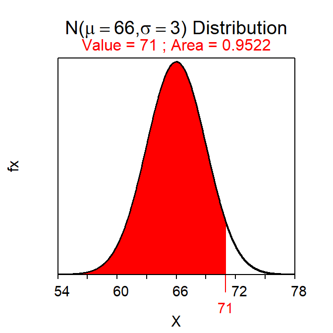
Figure 7.1: Calculation of the proportion of individuals on a \(N(66,3)\) with a value less than 71.
The proportion of students in this population that have a height greater than 68 inches is computed with (note use of lower.tail=FALSE)
( distrib(68,mean=66,sd=3,lower.tail=FALSE) )which produces Figure 7.2. Thus, approximately 25.2% of students in this population have a height greater than 68 inches.
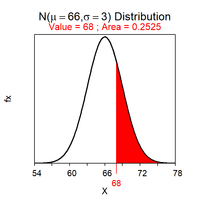
Figure 7.2: Calculation of the proportion of individuals on a \(N(66,3)\) with a value greater than 68.
If a question is a “Forward-Right” then you must include lower.tail=FALSE in distrib().
Finding the area between two particular values is a bit more work. To answer “between”-type questions, the area less than the smaller of the two values is subtracted from the area less than the larger of the two values. This is illustrated by noting that two values split the area under the normal curve into three parts – A, B, and C in Figure 7.3. The area between the two values is B. The area to the left of the larger value corresponds to the area A+B. The area to the left of the smaller value corresponds to the area A. Thus, subtracting the latter from the former leaves the “in-between” area B (i.e., (A+B)-A = B).
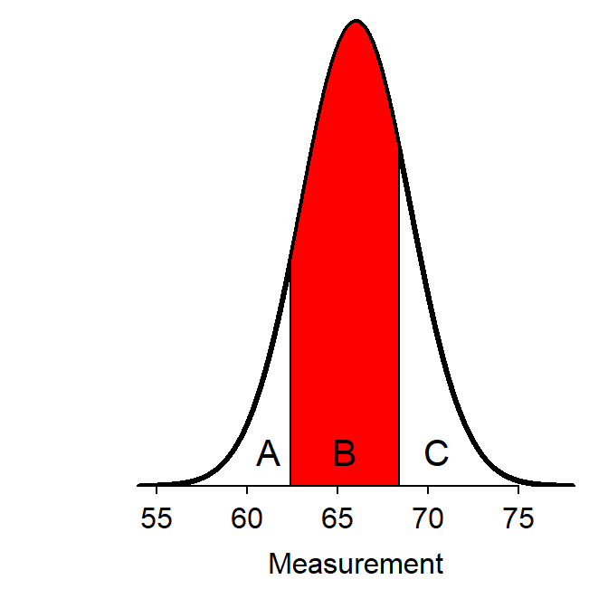
Figure 7.3: Schematic representation of how to find the area between two \(Z\) values.
For example, the area between 62 and 70 inches of height is found below. Thus, 81.8% of students in this population have a height between 62 and 70 inches.
( AB <- distrib(70,mean=66,sd=3) ) # left-of 70( A <- distrib(62,mean=66,sd=3) ) # left-of 62AB-A # between 62 and 70#R> [1] 0.8175776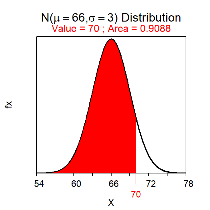
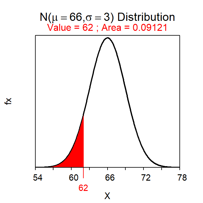
Figure 7.4: Calculation of the areas less than 70 inches (Left) and 62 inches (Right).
The area between two values is found by subtracting the area less than the smaller value from the area less than the larger value.
The area under the normal distribution is a proportion (of a whole) and should be presented in decimal form rounded to three decimal places (e.g., 0.734).
A percentage is a proportion that has been multiplied by 100. Percentages should generally be rounded to one decimal place (e.g., 73.4%) or one significant digit for very small values (e.g., 0.007%).
7.2 Reverse Calculations
Reverse questions also use distrib(), though the first argument is now the given percentage, though it must be entered as a proportion. The calculation is treated as a “reverse” question only when type="q" is also given to distrib().32 For example, the height that has 20% of all students shorter is computed with
( distrib(0.20,mean=66,sd=3,type="q") )which produces Figure 7.5. Thus, the shortest 20% of students are less than 63.5 inches tall.
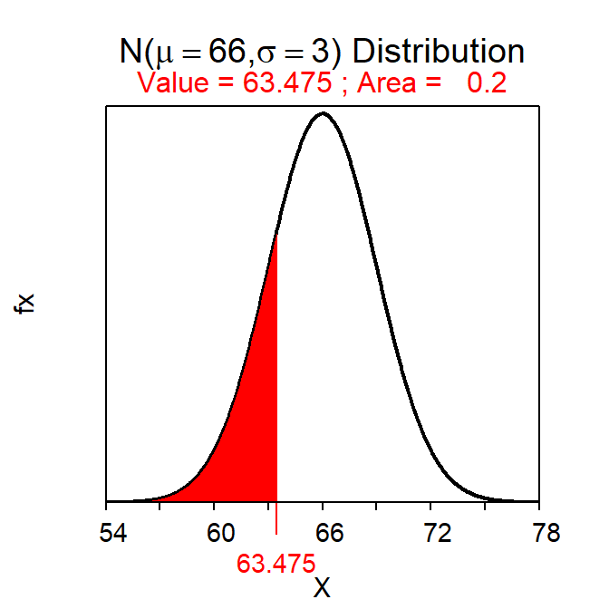
Figure 7.5: Calculation of the height with 20% of all students shorter.
“Greater than” reverse questions are computed by also including lower.tail=FALSE. For example, the tallest 10% of the population of students is computed with
( distrib(0.10,mean=66,sd=3,type="q",lower.tail=FALSE) )which produces Figure 7.6. Thus, the tallest 10% of students are taller than 69.8 inches.
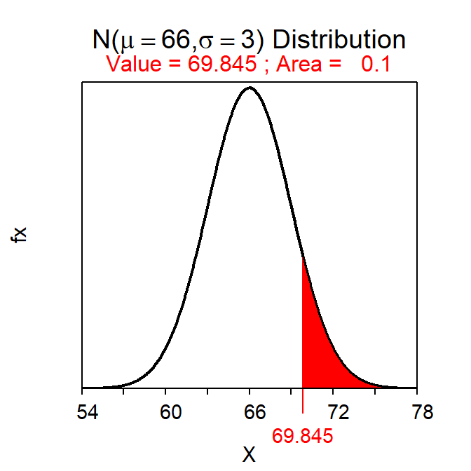
Figure 7.6: Calculation of the height with 10% of all students taller.
For “Reverse” normal distribution questions you MUST use type="q" in distrib(). If the question is a “Reverse-Right” then you must also include lower.tail=FALSE in distrib().
“Between” questions can only be easily handled if the question is looking for endpoint values that are symmetric about μ. In other words, the question must ask for the two values that contain the “most common” proportion of individuals. For example, suppose that you were asked to find the most common 80% of heights. This type of question is handled by converting this “symmetric between” question into two “less than” questions. For example, in Figure 7.7 the area D is the symmetric area of interest. If D is 0.80, then C+E must be 0.20.33 Because D is symmetric about μ, C and E must both equal 0.10. Thus, the lower bound on D is the value that has 10% of all values smaller. Similarly, because the combined area of C and D is 0.90, the upper bound on D is the value that has 90% of all values smaller. This question has now been converted from a “symmetric between” to two “less than” questions that can be answered exactly as shown above.
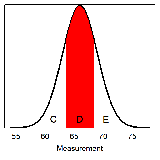
Figure 7.7: Depiction of areas in a reverse between type normal distribution question.
For example, the two heights that have a symmetric 80% of individuals between them are 62.2 and 69.8 inches as computed below.
( distrib(0.10,mean=66,sd=3,type="q") )
( distrib(0.90,mean=66,sd=3,type="q") )
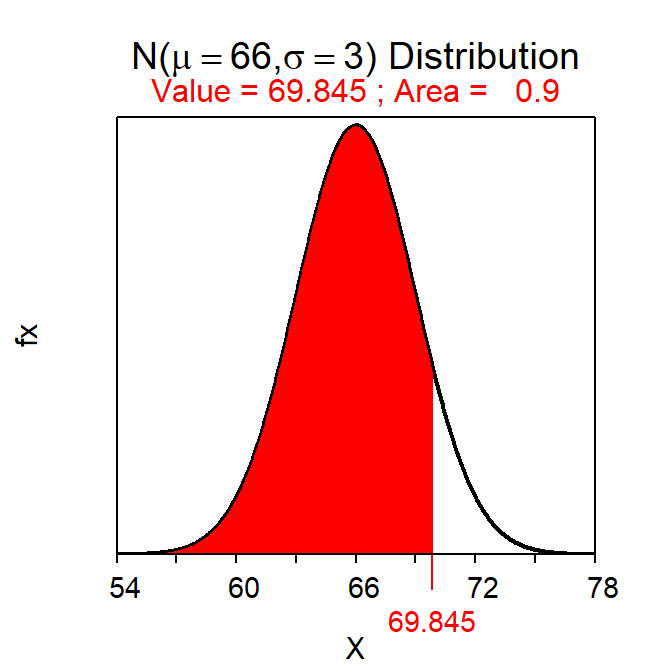
Figure 7.8: Calculations for the two values with an area of 80% between them.
For “Reverse-Between” questions you must convert the symmetric between area to two “left-of” areas and then perform two “Reverse-Left” questions with those areas.
Make sure to include appropriate units for the answers to “Reverse” questions.
7.3 Example Calculations
Suppose (as in Section 6.4) that the total miles driven per week by a particular person is normally distributed with a mean of 160 miles and a standard deviation of 25 miles. Use this information to answer the following questions.
- What percentage of weeks does the driver drive more than 125 miles?
- 91.9% – This is a Forward-Right question because a value of “X” is given and we should shade to the right (i.e., “more than”). This percentage is computed with
( distrib(125,mean=160,sd=25,lower.tail=FALSE) )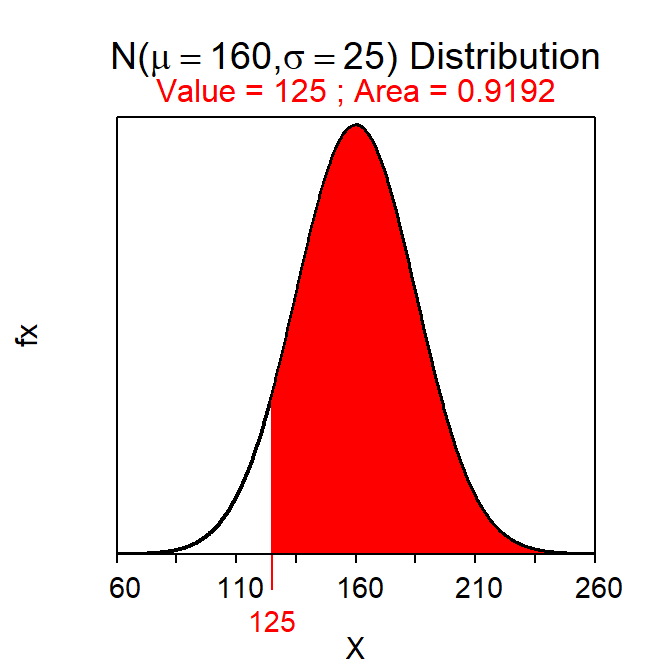
- What is the miles driven for the 25% of weeks with the fewest miles driven?
- Less than 143.1 miles – This is a Reverse-Left question because a percentage is given and we should shade to the left (i.e., “fewest”). This value is computed with
( distrib(0.25,mean=160,sd=25,type="q") )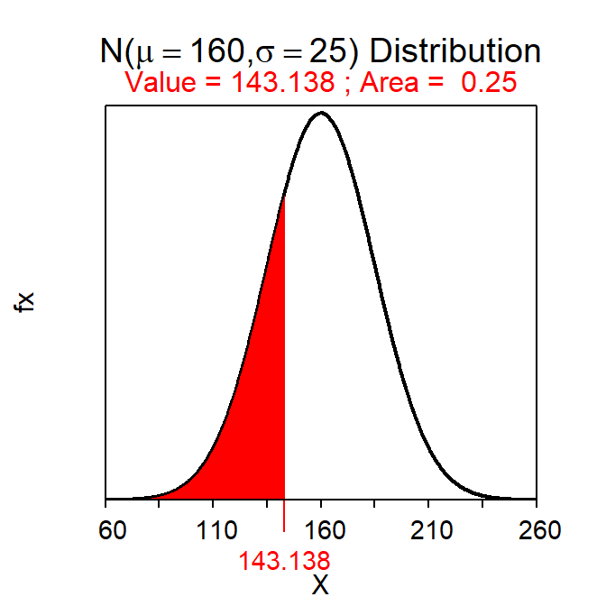
- What is the miles driven for the 5% of weeks with the most miles driven?
- More than 201.1 miles – This is a Reverse-Right question because a percentage is given and we should shade to the right (i.e., “most”). This value is computed with
( distrib(0.05,mean=160,sd=25,type="q",lower.tail=FALSE) )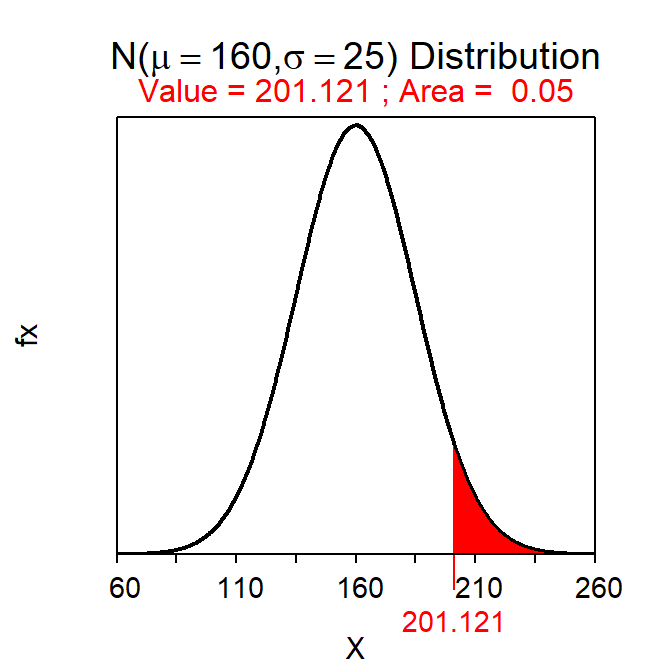
- What percentage of weeks does the driver drive between 75 and 100 miles?
- 0.8% – This is a Forward-Between question because two values of “X” are given and we should shade between the two values. This percentage is computed by finding the difference of the two areas provided from the following
( AB <- distrib(100,mean=160,sd=25) )
( A <- distrib(75,mean=160,sd=25) )
AB-A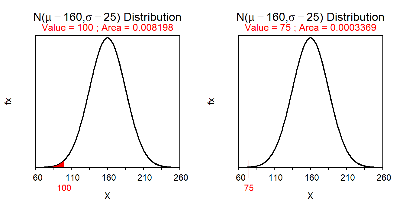
- What is the most common 60% of miles driven?
- Between 139.0 and 181.0 miles – This is a Reverse-between question because a percentage is given and we should shade in between (i.e., “most common”). These values are computed with
( distrib(0.2,mean=160,sd=25,type="q") )
( distrib(0.8,mean=160,sd=25,type="q") )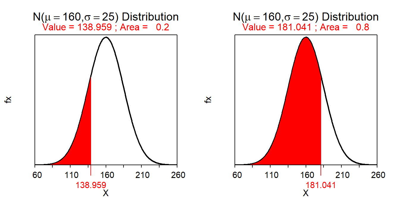
7.4 Standardization and Z-Scores
An individual that is 59 inches tall is 7 inches shorter than average if heights are N(66,3). Is this a large or a small difference? Alternatively, this same individual is \(\frac{-7}{3}\) = -2.33 standard deviations below the mean. Thus, a height of 59 inches is relatively rare in this population because few individuals are more than two standard deviations away from the mean.34 As seen here, the relative magnitude that an individual differs from the mean is better expressed as the number of standard deviations that the individual is away from the mean.
Values are “standardized” by changing the original scale (inches in this example) to one that counts the number of standard deviations (i.e., σ) that the value is away from the mean (i.e., μ). For example, with the height variable above, 69 inches is one standard deviation above the mean, which corresponds to +1 on the standardized scale. Similarly, 60 inches is two standard deviations below the mean, which corresponds to -2 on the standardized scale. Finally, 67.5 inches on the original scale is one half standard deviation above the mean or +0.5 on the standardized scale.
The process of computing the number of standard deviations that an individual is away from the mean is called standardizing. Standardizing is accomplished with
\[ \text{Z} = \frac{``\text{value"}-``\text{center"}}{``\text{dispersion"}} \]
or, more specifically,
\[ \text{Z} = \frac{\text{x}-\mu}{\sigma} \]
For example, the standardized value of an individual with a height of 59 inches is Z=\(\frac{59-66}{3}\)=-2.33. Thus, this individual’s height is 2.33 standard deviations below the average height in the population.
Standardized values (Z) follow a N(0,1). Thus, N(0,1) is called the “standard normal distribution.” The relationship between X and Z is one-to-one meaning that each value of X converts to one and only one value of Z. This means that the area to the left of X on a N(μ,σ) is the same as the area to the left of Z on a N(0,1). This one-to-one relationship is illustrated in Figure 7.9 using the individual with a height of 59 inches and Z=-2.33.
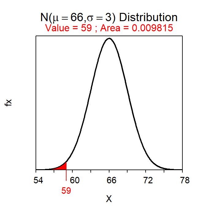
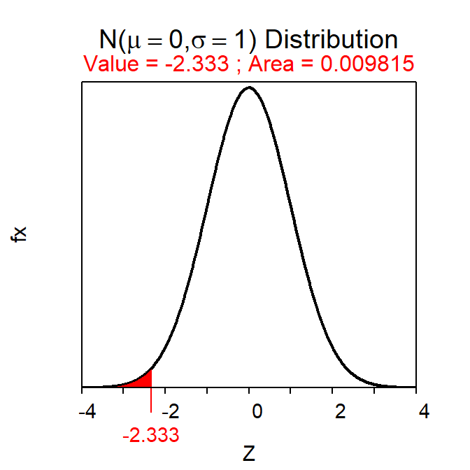
Figure 7.9: Plots depicting the area to the left of 59 on a N(66,3) (Left) and the area to the right of the corresponding Z-score of Z=-2.333 on a N(0,1) (Right). Note that the x-axis scales are different.
The standardized scale (i.e., z-scores) represents the number of standard deviations that a value is from the mean.