Module 16 Confidence Regions - Extension
In Module 15 the concept, calculation, and interpreation of confidence regions were introduced. In this module, some miscellaneous relationships and extensions of that material are introduced.
16.1 Confidence Intervals and Precision
The width of a confidence interval explains how precisely the parameter is estimated.63 More specifically, narrow intervals represent precise estimates of the parameter, whereas wide intervales represent imprecise estimates of the parameter.
The width of a confidence interval is directly related to the margin-of-error64 which depends on (1) the standard error and (2) the scaling factor. As either of these two items gets smaller (while holding the other constant), the width of the confidence interval gets smaller.
A small standard error means that sampling variability is low and precision is high. Smaller standard errors are obtained only by increasing the sample size. A smaller standard deviation would also result in a smaller SE, but the standard deviation cannot be made smaller (i.e., it is an inherent characteristic of the population).
A smaller scaling factor is obtained by reducing the level of confidence. For example, a 90% confidence interval uses a Z* of ±1.645, whereas a 95% confidence interval uses a Z* of ±1.960. Thus, decreasing the confidence level narrows the CI. However, reducing the level of confidence will also increase the number of confidence intervals that do not contain the parameter. Thus, reducing the level of confidence may not be the best choice for narrowing the confidence interval.
16.2 Sample Size Calculations
As noted in the previous module, the portion of the confidence interval to the right of the ± symbol is called the margin-of-error (ME). Thus,
\[ \text{ME} = \text{Z}^{*}\times\frac{\sigma}{\sqrt{\text{n}}} \]
This margin-of-error formula can be solved for n.
\[\begin{split} \text{ME} &= \text{Z}^{*}\times\frac{\sigma}{\sqrt{\text{n}}} \\ \sqrt{\text{n}} &= \frac{\text{Z}^{*}\times\sigma}{\text{ME}} \\ \text{n} &= \left(\frac{\text{Z}^{*}\times\sigma}{\text{ME}}\right)^{2} \\ \end{split} \]
This formula can be used to find the n required to estimate μ within ± ME units with C% confidence assuming that σ is known.
For example, suppose that one wants to determine n required to estimate the mean length of fish in Square Lake to within 5 mm with 90% confidence knowing that the population standard deviation is 34.91. From this, ME=5, σ=34.91, and Z*=1.645 (found previously for 90% confidence).65 Thus, n = \(\left(\frac{1.645\times34.91}{5}\right)^{2}\) = 131.91. Therefore, a sample of at least 132 fish from Square Lake should be taken to meet these constraints.
Sample size calculations are always rounded up to the next integer because rounding down would produce a sample size that does not meet the desired criteria.
The margin-of-error and confidence level in these calculations need to come from the researcher’s beliefs about how much error they can live with (i.e., chance that a confidence interval does not contain the parameter) and how precise their estimate of the mean needs to be (i.e., the ME they desire). Values for σ are rarely known in practice (because it is a parameter) and estimates from preliminary studies, previous similar studies, similar populations, or best guesses are often used instead. In practice, a researcher will often prepare a graph with varying values of σ to make an informed decision of what sample size to choose.
16.3 Inference Type Relationship
An alternative conceptualization of confidence intervals can show how confidence regions and hypothesis tests are related. This conceptualization rests on considering the sample means that would be “reasonable to see” from populations with various values of μ. A graphic is constructed below using the Square Lake population as an example and assuming that σ is known (=31.49), n=50, and 95% CIs are used.
First, compute the most common 95% of sample means assuming that μ=70; i.e., 70±1.960\(\frac{31.49}{\sqrt{50}}\) or (61.27,78.73). This range is plotted as a vertical rectangle centered on μ=70 (left-most rectangle) in Figure 16.1-Left. Next, compute and plot the same range for a slightly larger μ (e.g., with μ=71, plot (62.27,78.73)). Then repeat these steps for sequentially larger values of μ until a plot similar to Figure 16.1-Left is constructed.
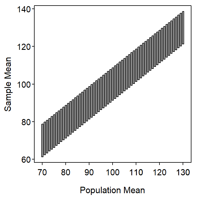
Figure 16.1: Range (95%) of sample means that would be produced by particular population means in the Square Lake fish length example.
Consider very carefully what Figure 16.1-Left represents. The vertical rectangles represent the ranges of the most common 95% of sample means (values read from the y-axis) that will be produced for a particular population mean (value read from the x-axis). In essence, each vertical line represents the sample means that are likely to be observed from a population with a given population mean (x-axis).
Now suppose that \(\bar{\text{x}}\)=100.04 (Table 2.2). Draw a horizontal line across Figure 16.1 at this value and then draw vertical lines down from where the horizontal line first enters and last leaves the band of possible sample means (Figure 16.2). The x-axis values that these vertical lines intercept are an approximate 95% CI for μ.
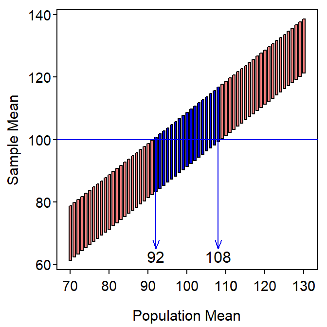
Figure 16.2: Range (95%) of sample means that would be produced by particular population means in the Square Lake fish length example with the ranges intercepted by \(\bar{\text{x}}\)=100.04 mm.
The actual confidence interval computed in Module 16 was (91.27,108.73), which compares favorably to the (92,108) from Figure 16.2. The approximation here will only as close as the intervals used to construct the rectangles (i.e., 1.0 mm were used here). More importantly, this graphical representation illustrates that a confidence interval (or region, more generally) consists of population means that are likely to produce the observed sample mean. Thus, a confidence region represents possible null hypothesized population means that WOULD NOT BE rejected during hypothesis testing.
A confidence region represents null hypothesized values that would NOT be rejected.
Be clear that this statement is about precision. We cannot usually speak to accuracy because the true value of the parameter is usually unknown.↩︎
More specifically the width of a confidence interval is two tmes the margin-of-error.↩︎
Strictly, Z*=±1.645, but the sign is inconsequential due to squaring in the sample size formula.↩︎