Module 28 t-Tests in R
In Modules 18 and 19 you learned the theory and how to perform the calculations required to complete the 11 steps of a hypothesis test (Section 17.1) for 1- and 2-sample t-tests. In this module, you will learn how to perform the required calculations from raw data using R.109
28.1 1-Sample t-Test
28.1.1 1-Sample t-Test in R
If raw data exist, the calculations for a 1-Sample t-test can be efficiently computed with t.test(). t.test() requires a formula of the form ~qvar, where qvar is the quantitative variable, as the first argument; the corresponding data frame in data=; the null hypothesized value for μ in mu=; the type of alternative hypothesis in alt= (can be alt="two.sided" (the default), alt="less", or alt="greater"); and the level of confidence as a proportion in conf.level= (defaults to 0.95). If the sample size is less than 40 then you may also need to construct a histogram as described in Section 25.1.2 to assess the shape of the distribution.
28.1.2 Example - Crab Body Temperature
Below are the 11 steps for completing a full hypothesis test (Section 17.1) for the following situation:
A marine biologist wants to determine if the body temperature of crabs exposed to ambient air temperature is different than the ambient air temperature. The biologist exposed a sample of 25 crabs to an air temperature of 24.3oC for several minutes and then measured the body temperature of each crab (shown below). Test the biologist’s question at the 5% level.
22.9,22.9,23.3,23.5,23.9,23.9,24.0,24.3,24.5,24.6,24.6,24.8,24.8,
25.1,25.4,25.4,25.5,25.5,25.8,26.1,26.2,26.3,27.0,27.3,28.1
Note that these data were entered into a data frame called CrabTemps.csv as discussed in Section 23.1.1 and that the R code used for this example is shown in the “R Code and Results” subsection below the 11 steps.
- α = 0.05.
- H0: μ = 24.3oC vs. HA: μ ≠ 24.3oC, where μ is the mean body temperature of ALL crabs.
- A 1-Sample t-Test is required because …
- a quantitative variable (temperature) was measured,
- individuals from one group (or population) were considered (an ill-defined population of crabs), and
- σ is UNknown.
- The data appear to be part of an experimental study (the temperature was controlled) with no suggestion of random selection of individuals.
- The assumptions are met because
- n = 25 ≥ 15 and the sample distribution of crab temperatures appears to be only slightly right-skewed (Figure 28.1) and
- σ is UNknown.
- x̄ = 25.0oC (Table 28.1).
- t = 2.713 with 24 df (Table 28.1).
- p-value = 0.0121 (Table 28.1).
- Reject H0 because the p-value < α.
- It appears that the average body temperature of ALL crabs is greater than the ambient temperature of 24.3oC.
- I am 95% confident that the mean body temperature of ALL crabs is between 24.5oC and 25.6oC (Table 28.1).
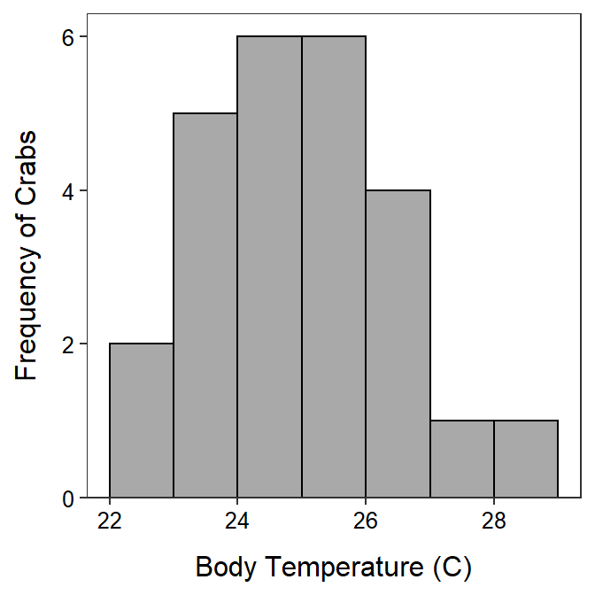
Figure 28.1: Histogram of the body temperatures of crabs exposed to an ambient temperature of 24.3oC.
| t = 2.7128, df = 24, p-value = 0.01215 |
| 95 percent confidence interval: |
| 24.47413 25.58187 |
| sample estimates: |
| mean of x |
| 25.028 |
R Appendix:
df <- read.csv("CrabTemps.csv")
ggplot(data=df,mapping=aes(x=ct)) +
  geom_histogram(boundary=0,binwidth=1,color="black",fill="darkgray") +
  labs(y="Frequency of Crabs",x="Body Temperature (C)") +
  scale_y_continuous(expand=expansion(mult=c(0,0.05))) +
  theme_NCStats()
( ct.t <- t.test(~ct,data=df,mu=24.3,conf.level=0.95) )
28.2 2-Sample t-Test
In Module 19 you learned about the theory underlying a 2-sample t-test and how to perform the calculations required to complete the 11 steps of a hypothesis test (Section 17.1). In this module, you will learn how to perform the required calculations from raw data using R. You will also be asked to complete the full 11-steps for a 2-sample t-test.
28.2.1 Data Format
The data used in this reading are the biological oxygen demand (BOD) measurements from either the inlet or outlet to an aquaculture facility. These data are in BOD.csv (data, meta) and are loaded into R below.
aqua <- read.csv("BOD.csv")Data must be in stacked format (as described in Section 23.1.1) for a 2-Sample t-Test. Stacked data has measurements in one column and group labels for the measurement in another column. Thus, each row corresponds to a measurement and the group for one individual. The BOD data are stacked because each row corresponds to one individual (a water sample) with one column of (BOD) measurements and another column for which group the individual belongs.
headtail(aqua)#R> BOD src
#R> 1 6.782 inlet
#R> 2 5.809 inlet
#R> 3 6.849 inlet
#R> 18 8.545 outlet
#R> 19 8.063 outlet
#R> 20 8.001 outlet28.2.2 Levene’s Test
Before conducting a 2-Sample t-Test, the assumption of equal population variances must be tested with Levene’s test. Levene’s test is computed with levenesTest(), where the first argument is a formula of the form qvar~cvar, where qvar represents the quantitative response variable and cvar represents the group factor variable.110 The data.frame containing qvar and cvar is given in data=. The results of the following code are shown in Table 28.2 and interpreted in the example analysis below.
levenesTest(BOD~src,data=aqua)28.2.3 Histograms
If the combined sample size for the two groups is less than 40 than histograms for both groups must be made to address the assumptions of normality before continuing with a 2-sample t-test. Separating histograms by groups was discussed in Section 25.2.1. The results of the following code are shown in Figure 28.2 and interpreted in the example analysis below.
ggplot(data=aqua,aes(x=BOD)) +
  geom_histogram(binwidth=0.5,boundary=0,color="black",fill="lightgray") +
  scale_y_continuous(expand=expansion(mult=c(0,0.05))) +
  labs(x="Biological Oxygen Demand",y="Frequency of Sites") +
  theme_NCStats() +
  facet_wrap(vars(src))
28.2.4 2-Sample t-Test in R
A 2-Sample t-Test is computed with t.test(), where the first argument is the same formula as in levenesTest() (and, thus, same data=). Additionally, the following arguments may need to be specified.
mu=: The specific value in H0. For a 2-Sample t-Test this is usually 0, which is the default.alt=: A string that indicates the type of HA (i.e.,"two.sided"(default),"greater", or"less").conf.level=: The level of confidence (default is0.95) used for the confidence region of μ1-μ2.var.equal=: A logical value that indicates whether the two population variances should be considered equal or not. IfTRUE, then the pooled sample variance is calculated and used in the standard error. The default isFALSEwhich assumes UNequal variances.
R computes the difference among groups as the alphabetically “first” level minus the alphabetically “second” level. For example, if the two levels are inlet and outlet, then R will compute x̄inlet-x̄outlet. You should consider this when you are constructing your hypotheses. However, you can change the order of the levels by using levels= in factor() (as described in Section 25.3.1).
The results of the following code are shown in Table 28.3 and interpreted in the example analysis below.
t.test(BOD~src,data=aqua,var.equal=TRUE,alt="less",conf.level=0.90)
28.2.5 Example - BOD in Aquaculture Water
Below are the 11 steps of a hypothesis test (Section 17.1) for the following situation (which follows from above):
An aquaculture farm takes water from a stream and returns it to the stream after it has circulated through the fish tanks. The owner has taken steps to reduce the level of organic matter in the water released back into the stream. However, he is still concerned that water returned to the stream may contain heightened levels of organic matter. To determine if this is true, he took samples of water at the intake and, at other times, downstream from the outlet and recorded the biological oxygen demand (BOD) as a measure of the organics in the effluent (a higher BOD at the outlet would imply heightened levels of organics are being released to the stream). The owner’s data are recorded in BOD.csv. Test for any evidence (i.e., at the 10% level) to support the owner’s concern.
- α = 0.10.
- H0:μinlet-μoutlet=0 vs HA:μinlet-μoutlet<0, where μ is the mean BOD for this aquaculture facility and the subscript represent measurements at the inlet and outlet, respectively. [Negative differences represent larger values at the outlet, which implies that BOD is higher in the water released from the facility. Thus, HA represents the owner’s concern.]
- A 2-Sample t-Test is required because …
- a quantitative variable (BOD level) was measured,
- two groups are being compared (inlet and outlet), and
- the individuals in the groups were INdependent (note that it said that the outlet samples came from different times then the inlet samples).
- The data appear to be part of an observational study (the inlet and outlet groups were naturally occurring and were not groups created by the researcher) with no obvious randomization.
- The assumptions are met because …
- n = 20>15 and the histograms (Figure 28.2) are inconclusive about the shape because of the small sample size in each group (it appears that the
inletdata is not strongly skewed, whereas theoutletdata is skewed, which may invalidate the results of this hypothesis test; however, I continued to make a complete example), - individuals in the two groups are independent as discussed above, and
- the variances appear to be equal because the Levene’s test p-value (=0.5913; Table 28.2) is greater than α.
- n = 20>15 and the histograms (Figure 28.2) are inconclusive about the shape because of the small sample size in each group (it appears that the
- x̄inlet-x̄outlet = 6.65 - 8.69 = -2.03 (Table 28.3).
- t = -8.994 with 18 df (Table 28.3).
- p-value 0.00000002 (Table 28.3).
- H0 is rejected because the p-value < α.
- The average BOD is greater at the outlet than at the inlet to the aquaculture facility. Thus, the aquaculture facility appears to add to the biological oxygen demand of the water and the farmer’s concern is warranted.
- I am 90% confident that the mean BOD measurement at the outlet is AT LEAST 1.73 GREATER than the mean BOD measurement at the inlet (Table 28.3).
| Df | F value | Pr(>F) | |
|---|---|---|---|
| group | 1 | 0.2988958 | 0.5912891 |
| 18 |
| t = -8.994, df = 18, p-value = 2.224e-08 |
| 90 percent confidence interval: |
| -Inf -1.732704 |
| sample estimates: |
| mean in group inlet mean in group outlet |
| 6.6538 8.6873 |
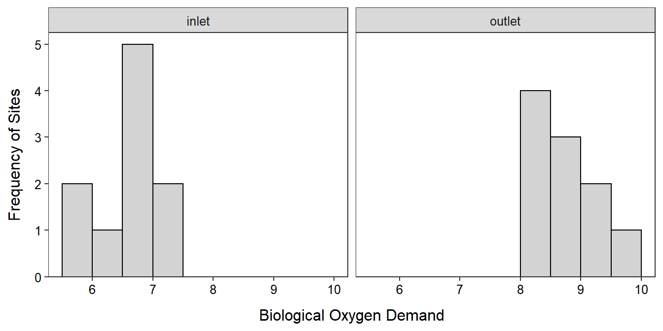
Figure 28.2: Histogram of the BOD measurements at the outlet and inlet of the aquaculture facility.
R Appendix
aqua <- read.csv("BOD.csv")
ggplot(data=aqua,aes(x=BOD)) +
  geom_histogram(binwidth=0.5,boundary=0,color="black",fill="lightgray") +
  scale_y_continuous(expand=expansion(mult=c(0,0.05))) +
  labs(x="Biological Oxygen Demand",y="Frequency of Sites") +
  theme_NCStats() +
  facet_wrap(vars(src))
levenesTest(BOD~src,data=aqua)
t.test(BOD~src,data=aqua,var.equal=TRUE,alt="less",conf.level=0.90)
28.3 Generic R Code
The following generic codes were used in this module and are provided here so that you can efficiently copy and paste them into your assignment. Note the following:
dfobjshould be replaced with the name of your data frame.qvarshould be replaced with the name of your quantitative variable.cvarshould be replaced with the name of your categorical variable.mu0is the population mean in H0.HAis replaced with"two.sided"for not equals,"less"for less than, or"greater"for greater than alternative hypotheses (HA).cnfvalis the confidence level as a proportion (e.g.,0.95).
Also examine the “R Function Guide” on the class Resources page for more guidance.
1-Sample t-Test
t.test(~qvar,data=dfobj,mu=mu0,alt=HA,conf.level=cnfval)2-Sample t-test
- Construct a Levene’s Test
levenesTest(qvar~cvar,data=dfobj)- Construct a 2-Sample t-Test
t.test(qvar~cvar,data=dfobj,alt=HA,conf.level=cnfval,var.equal=TRUE)