Module 2 Foundational Definitions
Statistical inference is the process of forming conclusions about a parameter of a population from statistics computed from individuals in a sample.4 Thus, understanding statistical inference requires understanding the difference between a population and a sample and a parameter and a statistic. And, to properly describe those items, the individual and variable(s) of interest must be identified. Understanding and identifying these six items is the focus of this module.
The following hypothetical example is used throughout this module. Assume that we are interested in the average length of 1015 fish in Square Lake. To illustrate important concepts in this module, assume that all information for all 1015 fish in this lake is known (Figure 2.1). In “real life” this complete information would not be known.
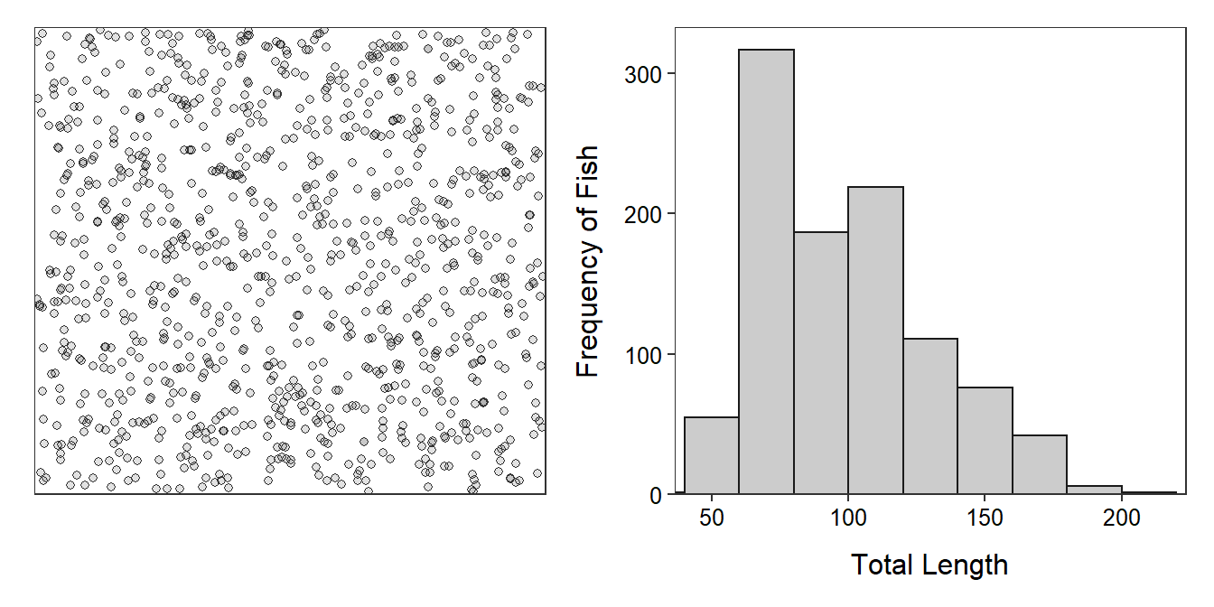
Figure 2.1: Schematic representation of individual fish (i.e., dots; Left) and histogram (Right) of the total length of the 1015 fish in Square Lake.
2.1 Definitions
The individual in a statistical analysis is one of the “items” examined by the researcher.5 Sometimes the individual is a person, but it may be an animal, a piece of wood, a location, a particular time, or an event. It is extremely important that you don’t always visualize a person when identifying a statistical individual. An individual in the Square Lake example is a fish because the researcher will examine a characteristic of each particular fish.
An individual is not necessarily a person.
The variable is the characteristic recorded about each individual. The variable in the Square Lake example is the length of each fish. In most studies, the researcher will record more than one variable. For example, the researcher may also record the fish’s weight, sex, age, time of capture, and location of capture. In this module, only one variable is considered, but in other modules two variables will be considered.
A population is ALL individuals of interest. In the Square Lake example, the population is all 1015 fish in the lake. The population should be defined as thoroughly as possible including qualifiers, especially those related to time and space, as necessary. This example is simple because Square Lake is so well defined; however, as you will see in the examples below, the population is often only well-defined by your choice of descriptors.
A parameter is a summary computed from ALL individuals in a population. In this module the summary will either be the mean or percentage. For example, the mean length (=98.06 mm) and standard deviation (=31.49 mm; Table 2.1) of ALL 1015 fish in Square Lake are both parameters.6 Parameters are ultimately what is of interest because interest is in all individuals in the population. However, in practice, parameters cannot be computed because the entire population cannot usually be “seen.” Summaries for parameters are preceded by “population”; e.g., population mean or population standard deviation.
| n | mean | sd | min | Q1 | median | Q3 | max |
|---|---|---|---|---|---|---|---|
| 1015 | 98.06 | 31.49 | 39 | 72 | 93 | 117 | 203 |
Populations and parameters can generally not be”seen.”
To learn something about a population that cannot usually be seen we must sample a subset of that population. The red dots in Figure 2.2 represent a random sample of n=50 fish from Square Lake (note that the sample size is usually denoted by n).
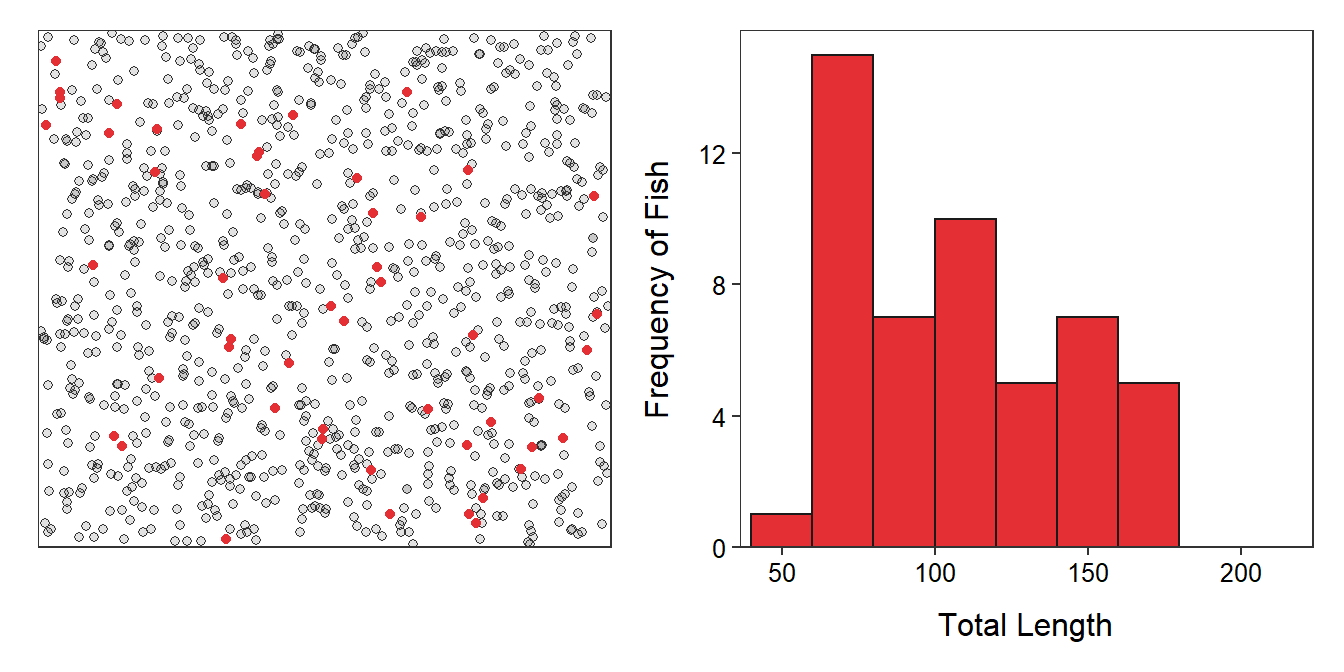
Figure 2.2: Schematic representation (Left) of a sample of 50 fish (i.e., red dots) from Square Lake and histogram (Right) of the total length of the 50 fish in this sample.
Summaries computed from individuals in a sample are called statistics. The summary for the statistic is always the same as that for the parameter; i.e., the statistic describes the sample in the same way that the parameter describes the population. For example, if mean was used for the parameter then the mean will be used for the statistic. Summaries for statistics are preceded by “sample”; e.g., sample mean or sample standard deviation.
Some statistics computed from the sample from Square Lake are shown in Table 2.2 and Figure 2.2. The sample mean of 107.5 mm is the best “guess” at the population mean. Not surprisingly from the discussion in Module 1, the sample mean does not perfectly equal the population mean.
| n | mean | sd | min | Q1 | median | Q3 | max |
|---|---|---|---|---|---|---|---|
| 50 | 107.5 | 34.26 | 57 | 77.25 | 107.5 | 134.75 | 171 |
A sample represents a population, a statistic represents (or is an estimate of) a parameter.
2.2 Performing an IVPPSS
In each statistical analysis it is important that you determine the Individual, Variable, Population, Parameter, Sample, and Statistic. First, determine what items you are actually going to look at; those are the individuals. Second, determine what is recorded about each individual; that is the variable. Third, ALL individuals is the population. Fourth, the summary (e.g., mean or percentage) of the variable recorded from ALL individuals in the population is the parameter.7 Fifth, the population usually cannot be seen, so only a few individuals are examined; those few individuals are the sample. Finally, the summary of the individuals in the sample is the statistic.
When performing an IVPPSS, keep in mind that parameters describe populations (note that they both start with “p”) and statistics describe samples (note that they both start with “s”). This can also be looked at from another perspective. A sample is an estimate of the population and a statistic is an estimate of a parameter. Thus, the statistic has to be the same summary (mean or percentage) from the sample as the parameter is from the population.
Example – Rabbits in Maine
 The IVPPSS process is illustrated for the following situation:
A University of New Hampshire graduate student (and Northland College alum) investigated habitat utilization by New England (Sylvilagus transitionalis) and Eastern (Sylvilagus floridanus) cottontail rabbits in eastern Maine in 2007. In a preliminary portion of his research he determined the percentage of “rabbit patches” that were inhabited by New England cottontails. He examined 70 “patches” and found that 53 showed evidence of inhabitance by New England cottontails.
- An individual is a rabbit patch in eastern Maine in 2007 (i.e., a rabbit patch is the “item” being sampled and examined).
- The variable is “evidence for New England cottontails (yes or no)” (i.e., the characteristic of each rabbit patch that was recorded).
- The population is ALL rabbit patches in eastern Maine in 2007.
- The parameter is the percentage of ALL rabbit patches in eastern Maine in 2007 that showed evidence for New England cottontails.8
- The sample is the 70 rabbit patches from eastern Maine in 2007 that were actually examined by the researcher.
- The statistic is the percentage of the 70 rabbit patches from eastern Maine in 2007 actually examined that showed evidence for New England cottontails. [In this case, the statistic would be \(\frac{53}{70}\)×100 or 75.7%.]
In the descriptions above, take note that the individual is very carefully defined (including stating a specific time (2007) and place (eastern Maine)), the population and parameter both use the word “ALL,” the sample and statistic both use the specific sample size (70 rabbits), and the parameter and statistics both use the same summary (i.e., percentage of patches that showed evidence of New England cottontails).
Example – Duluth Raptors
In some situations it may be easier to identify the sample first. From this, and realizing that a sample is always “of the individuals,” it may be easier to identify the individual. This process is illustrated in the following example, with the items listed in the order identified rather than in the traditional IVPPSS order.
The Duluth, MN Touristry Board is interested in the average number of raptors seen per year at Hawk Ridge.9 To determine this value, they collected the total number of raptors seen in a sample of years from 1971-2003.
- The sample is the 32 years between 1971 and 2003 at Hawk Ridge.
- An individual is a year (because a “sample of years” was taken) at Hawk Ridge.
- The variable recorded was the number of raptors seen in one year at Hawk Ridge.
- The population is ALL years at Hawk Ridge.10
- The parameter is the average number of raptors seen per year in ALL years at Hawk Ridge.
- The statistic is the average number of raptors seen in the 1971-2003 sample of years at Hawk Ridge.
Again, note that the individual is very carefully defined (including stating a specific time and place), the population and parameter both use the word “ALL,” the sample and statistic both use the specific sample size (32 years), and the parameter and statistics both use the same summary (i.e., average number of raptors).
- An individual is usually defined by a specific time and place. *Descriptions for population and parameter will always include the word “All.”
- Descriptions for sample and statistic will contain the specific sample size.
- Descriptions for parameter and statistic will contain the same summary (usually average/mean or proportion/percentage). However the summary is for a different set of individuals – the population for the parameter and the sample for the statistic.
2.2.1 Sampling Variability (Revisited)
It is instructive to once again (see Module 1) consider how statistics differ among samples. Table 2.3 and Figure 2.3 show results from three more samples of n=50 fish from the Square Lake population. The means from all four samples (including the sample in Table 2.2 and Figure 2.2) were quite different from the known population mean of 98.06 mm. Similarly, all four histograms were similar in appearance but slightly different in actual values. These results illustrate that a statistic (or sample) will only approximate the parameter (or population) and that statistics vary among samples. This sampling variability is one of the most important concepts in statistics and is discussed in great detail beginning in Module 11.
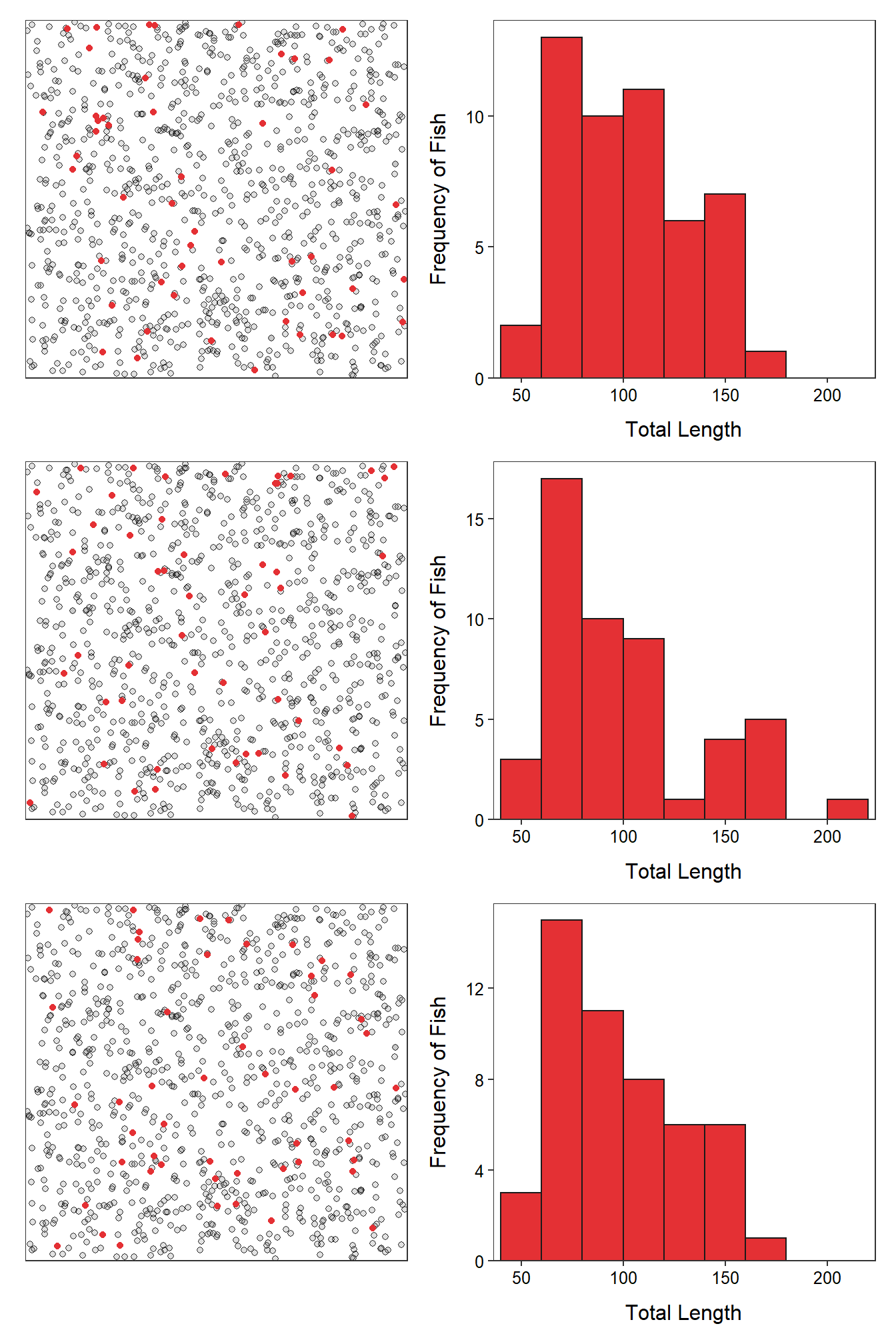
Figure 2.3: Schematic representation (Left) of three samples of 50 fish (i.e., red dots) from Square Lake and histograms (Right) of the total length of the 50 fish in each sample.
| n | mean | sd | min | Q1 | median | Q3 | max | |
|---|---|---|---|---|---|---|---|---|
| 2 | 50 | 100.48 | 31.87 | 45 | 78.25 | 99.5 | 120.00 | 180 |
| 3 | 50 | 99.40 | 38.28 | 47 | 69.00 | 90.5 | 113.75 | 203 |
| 4 | 50 | 98.14 | 32.26 | 45 | 71.25 | 87.0 | 121.50 | 174 |
Sampling Variability: The realization that no two samples are exactly alike. Thus, statistics computed from different samples will likely vary.
This example also illustrates that parameters are fixed values because populations don’t change. If a population does change, then it is considered a different population. In the Square Lake example, if a fish is removed from the lake, then the fish in the lake would be considered a different population. Statistics, on the other hand, vary depending on the sample because each sample consists of different individuals that vary (i.e., sampling variability exists because natural variability exists).
Parameters are fixed in value, while statistics vary in value.
2.3 Variable Types
The type of statistic that can be calculated is dictated by the type of variable recorded. For example, an average can only be calculated for quantitative variables (defined below). Thus, the type of variable should be identified immediately after performing an IVPPSS.
2.3.1 Variable Definitions
There are two main groups of variable types – quantitative and categorical (Figure 2.4). Quantitative variables are variables with numerical values for which it makes sense to do arithmetic operations (like adding or averaging).11 Categorical variables are variables that record which group or category an individual belongs.12 Within each main type of variable are two subgroups (Figure 2.4).
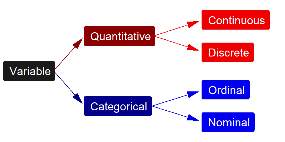
Figure 2.4: Schematic representation of the four types of variables.
The two types of quantitative variables are continuous and discrete variables. Continuous variables have an uncountable number of values. Discrete variables have a countable number of values. Typically, but not always, discrete variables are counts of items.
Continuous and discrete variables are easily distinguished by determining if it is possible for a value to exist between every two values of the variable. If a potential value can always be found between two values then the variable is continuous, otherwise it is discrete. For example, can there be between 2 and 3 ducks on a pond? No! Thus, the number of ducks is a discrete variable. Alternatively, can a duck weigh between 2 and 3 kg? Yes! Can it weigh between 2 and 2.1 kg? Yes! Can it weigh between 2 and 2.01 kg? Yes! You can see that this line of questions could continue forever; thus, duck weight is a continuous variable.
A quantitative variable is continuous if a possible value exists between every two values of the variable; otherwise, it is discrete.
The two types of categorical variables are ordinal and nominal. Ordinal variables have a natural order or ranking among the categories. Nominal variables have no order or ranking among the categories.
Ordinal and nominal variables are easily distinguished by determining if the order of the categories matters. For example, suppose that a researcher recorded a subjective measure of condition (i.e., poor, average, excellent) and the species of each duck. Order matters with the condition variable – i.e., condition improves from the first (poor) to the last category (excellent) – and some reorderings of the categories would not make sense – i.e., average, poor, excellent does not make sense. Thus, condition is an ordinal variable. In contrast, species (e.g., mallard, redhead, canvasback, and wood duck) is a nominal variable because there is no inherent order among the categories (i.e., any reordering of the categories also “makes sense”).
Ordinal means that an order among the categories exists (note “ord” in both ordinal and order).
The following are some issues to consider when identifying the type of a variable:
- Counts of numbers are discrete (quantitative) variables.
- Measurements are typically continuous (quantitative) variables.
- It does not matter how precisely quantitative variables are recorded when deciding if the variable is continuous or discrete. For example, the weight of the duck might have been recorded to the nearest kg. However, this was just a choice that was made, the actual values can be continuously finer than kg and, thus, weight is a continuous variable.
- The categories of a categorical variable are sometimes labeled with numbers. For example, 1=“Poor,” 3=“Fair,” and 5=“Good.” Don’t let this fool you into calling the variable quantitative.
- Rankings, ratings, and preferences are ordinal (categorical) variables.
- Categorical variables that consist of only two levels or categories will be labeled as a nominal variable (because any order of the groups makes sense). This type of variable is also often called “binomial.”
- Do not confuse “what type of variable” (answer is one of “continuous,” “discrete,” “nominal,” or “ordinal”) with “what type of variability” (answer is “natural” or “sampling”) questions.
Formal methods of inference are discussed beginning with Module 12.↩︎
Synonyms for individual are unit, experimental unit (usually used in experiments), sampling unit (usually used in observational studies), case, and subject (usually used in studies involving humans).↩︎
We will discuss how to compute and interpret each of these values in Module 4.↩︎
Again, parameters generally cannot be computed because all of the individuals in the population can not be seen. Thus, the parameter is largely conceptual.↩︎
Note that this population and parameter cannot actually be calculated but it is what the researcher wants to know.↩︎
This is a bit ambiguous but may be thought of as all years that Hawk Ridge has existed.↩︎
Synonyms for quantitative are measurement or numerical.↩︎
Synonyms for categorical are qualitative or attribute.↩︎