Module 19 SLR Summary

Specific parts of a full Simple Linear Regression (SLR) analysis were described in Modules 14-18. In this module, a workflow for a full analysis is offered and that workflow is demonstrated with several examples.

19.1 Suggested Workflow

The following is a process for fitting a SLR. Consider this process as you learn to fit SLR models, but don’t consider this to be a concrete process for all models.

1. Briefly introduce the study (i.e., provide some background for why this study is being conducted).
2. State the hypotheses to be tested.
3. Show the overall sample size.
4. Address the independence assumption.
   • If this assumption is not met then other analysis methods must be used.
5. Fit the untransformed full model with lm().
6. Check the other four assumptions for the untransformed model with assumptionCheck().
   • Check the linearity of the relationship with the residual plot.
   • Check homoscedasticity with the residual plot.
   • Check normality of residuals with an Anderson-Darling test and histogram of residuals.
   • Check outliers and influential points with the outlier test and residual plot.
7. If an assumption or assumptions are violated, then attempt to find a transformation where the assumptions are met.
   • Use trial-and-error with assumptionCheck(), theory (e.g., power or exponential functions), or experience to identify possible transformations for the response variable and, possibly, for the explanatory variable.
     • Attempt transformations with the response variable first.
     • Generally only ever transform the explanatory variable with logarithms.
   • If only an outlier or influential observation exists (i.e., linear, homoscedastic, and normal residuals) and no transformation corrects the “problem,” then consider removing that observation from the data set.
   • Fit the full model with the transformed variable(s) or reduced data set.
8. Construct an ANOVA table for the full model with anova() and interpret the overall F-test.
9. Summarize findings with coefficient results and confidence intervals with cbind(coef(),confint()).
10. Create a summary graphic of the fitted line with 95% confidence band using ggplot().
11. Make predictions with predict(), if desired.
12. Write a succinct conclusion of your findings.

 

19.2 Climate Change Data (No Transformation)

Climate researchers examined the relationship between global temperature anomaly and the concentration of CO₂ in the atmosphere. Temperature anomaly data were recorded as the Global Land-Ocean Temperature Index from the Goddard Institute of Space Studies (GISTEMP) in units of 1/100^oC increase above the 1950-1980 mean. The CO₂ data are from The Earth System Research Laboratory of the National Oceanic and Atmospheric Administration (ESRL-NOAA). Specifically, these data are a record of annual mean atmospheric CO₂ concentration at Mauna Loa Observatory Hawaii, which constitute the longest continuous record of atmospheric CO₂ concentrations. This remote location at high altitude in Hawaii was chosen because it is relatively unaffected by any local emissions and so is representative of the global concentration of a well-mixed gas like CO₂. These observations were started by C. David Keeling of the Scripps Institution of Oceanography in March of 1958 and are often referred to as the Keeling Curve. Data are reported as a dry mole fraction defined as the number of molecules of carbon dioxide divided by the number of molecules of dry air multiplied by one million (ppm). Our goal here is to determine if the variability in the temperature anomaly records can be reasonably explained by the CO₂ values in the same year.

The statistical hypotheses to be examined are

\[ \begin{split} \text{H}_{\text{0}}&: ``\text{no relationship between temperature anomaly and CO2 values''} \\ \text{H}_{\text{A}}&: ``\text{is a relationship between temperature anomaly and CO2 values''} \\ \end{split} \]

Data were recorded for 32 years. The data between years is likely not independent as knowing the temperature anomaly and CO₂ values in any given year likely are a good indicator of the values in the next year. This temporal dependence should probably be included in the analysis. However, these data are recorded on an annual basis and it does not make much sense to include only a random sample of years. Thus, to better understand the relationship between these two variables, I will continue with this analysis assuming independence.

The assumptions are met as the residual plots show no obvious curvature or funneling (Figure 19.1-Right), the histogram of residuals is not strongly skewed (Figure 19.1-Left; Anderson-Darling p=0.4313), and there are no obvious outliers (p>1). Thus, the analysis can continue without any transformations.

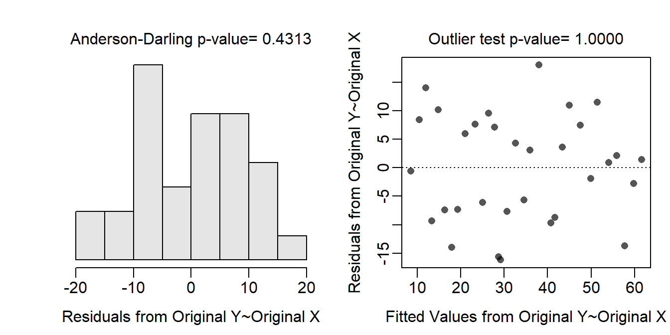
Figure 19.1: Histogram of residuals (Left) and residual plot (Right) for a simple linear regression of temperature anomaly on CO2 data.

 

The temperature anomaly and CO₂ data appear to be significantly related (p<0.00005; Table 19.1). In fact, 74.1% of the variability in the temperature anomaly is explained by knowing the value of the CO₂ concentration.

 

Table 19.1: ANOVA table for simple linear regression of temperature anomaly on CO2 data.

	Df	Sum Sq	Mean Sq	F value	Pr(>F)
CO2	1	7717.1	7717.1	85.918	0
Residuals	30	2694.6	89.8

 

In fact, it appears that as as the CO₂ levels increase by 1 ppm then the mean temperature anomaly increases by between 0.80 and 1.26 1/100^oC (Table 19.2; Figure 19.2).

 

Table 19.2: Intercept and slope, along with 95% confidence intervals, for simple linear regression of temperature anomaly on CO2 data.

	Est	2.5 %	97.5 %
(Intercept)	-338.25	-420.24	-256.25
CO2	1.03	0.80	1.26

 

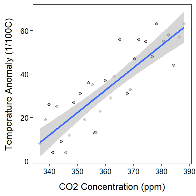
Figure 19.2: Scatterplot of temperature anomaly versuse CO2 concentration with the best-fit line and 95% confidence band superimposed.

 

Finally, the predicted mean temperature anomaly for all times when the CO₂ concentration was 360 ppm is between 29.2 and 36.0 1/100^oC.

In conclusion, a significantly positive and strong relationship was found between the mean temperature anomaly and the global CO₂ concentration. A model was developed from this relationship that can be used to predict the temperatuare anomaly from the CO₂ concentration.

R Code and Results

cc <- read.csv("http://derekogle.com/NCMTH107/modules/CE/GSI_data.csv")
str(cc)
lm.cc <- lm(Temp~CO2,data=cc)
assumptionCheck(lm.cc)

anova(lm.cc)
rSquared(lm.cc)
cbind(Est=coef(lm.cc),confint(lm.cc))
ggplot(data=cc,mapping=aes(x=CO2,y=Temp)) + 
  geom_point(pch=21,color="black",fill="lightgray") + 
  labs(x="CO2 Concentration (ppm)",y="Temperature Anomaly (1/100C)") + 
  theme_NCStats() + 
  geom_smooth(method="lm")

nd <- data.frame(CO2=360)
predict(lm.cc,newdata=nd,interval="confidence")

 

19.3 Forest Allometrics (Transformation)

Understanding the carbon dynamics in forests is important to understanding ecological processes and managing forests. The amount of carbon stored in a tree is related to tree biomass. Measuring the biomass of a tree is a tedious process that also results in the harvest (i.e., death) of the tree. However, biomass is often related to other simple metrics (e.g., diameter-at-breast-height (DBH) or tree height) that can be made without harming the tree. Thus, forest scientists have developed a series of equations (called allometric equations) that can be used to predict tree biomass from simple metrics for a variety of trees in a variety of locations.

The Miombo Woodlands is the largest continuous dry deciduous forest in the world. It extends across much of Central, Eastern, and Southern Africa including parts of Angola, the Democratic Republic of Congo, Malawi, Mozambique, Tanzania, Zambia, and Zimbabwe. The woodlands are rich in plant diversity and have the potential to contain a substantial amount of carbon. There is, however, significant uncertainty in the amount of biomass carbon in the Miombo Woodlands. The objective of this study (Kuyah et al. 2016) is to develop allometric equations that can be used to reliably estimate biomass of trees in the Miombo Woodlands so that biomass carbon can be more reliably estimated.

Trees for building allometric models were sampled from three 10 km by 10 km sites located in the districts of Kasungu, Salima, and Neno. A total of 88 trees (33 species) were harvested from six plots in Kasungu, seventeen plots in Salima, and five plots in Neno. The DBH (cm) of each tree was measured using diameter tape. Each tree was felled by cutting at the lowest possible point using a chainsaw. The length (m) of the felled tree was measured along the longest axis with a measuring tape. This measurement was used as the total tree height in the analysis. Felled trees were separated into stem, branches, and twigs (leaves and small branches). Total biomass (kg) of the tree (above-ground biomass; AGB) and the separate biomasses (kg) of the stems, branches, and twigs was recorded. The data are stored in TreesMiombo.csv (data, meta). This analysis will attempt to predict AGB from DBH.

The statistical hypotheses to be examined are

\[ \begin{split} \text{H}_{\text{0}}&: ``\text{no relationship between above ground biomass and diameter at breast height''} \\ \text{H}_{\text{A}}&: ``\text{is a relationship between above ground biomass and diameter at breast height''} \\ \end{split} \]

There is some concern over independence because some of the trees presumably came from the same plot and it is possible that one tree might have an impact on another tree. That impact may have been on the overall growth of the tree through density-dependent factors, but it is hard to imagine how one tree could effect another tree with respect to the relationship between above ground biomass and diameter at breast height. Thus, I will continue with this analysis assuming independence.

The residual plot (Figure 19.3-Right) indicates a lack of linearity and homoscedasticity as there is both a clear curve and funnel present. There also appears to be a lack of normality in the residuals (Anderson-Darling p=0.0041) and the presence of outliers (outlier test p<0.00005). These results all indicate that a transformation should be explored.

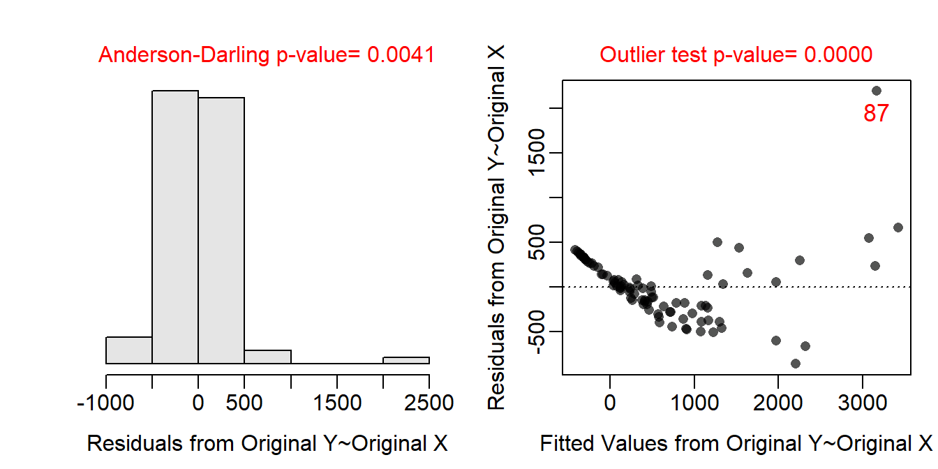
Figure 19.3: Histogram of residuals (Left) and residual plot (Right) for a simple linear regression of above ground biomass on diameter at breast height for trees from the Miombo Woodlands.

 

Allometric relationships between weights (i.e., biomass) and lengths (i.e., height) tend to follow a power function, which can be linearized by log-transforming both variables. When both variables were transformed the relationship was largely linear and homoscedastic (Figure 19.4-Right), the residuals appeared to be normal (Anderson-Darling p=0.4463; Figure 19.4-Left), and no outliers were present (outlier test p>1). Thus, the linear regression model was fit to the log-log transformed data as all assumptions were met on this scale.

 

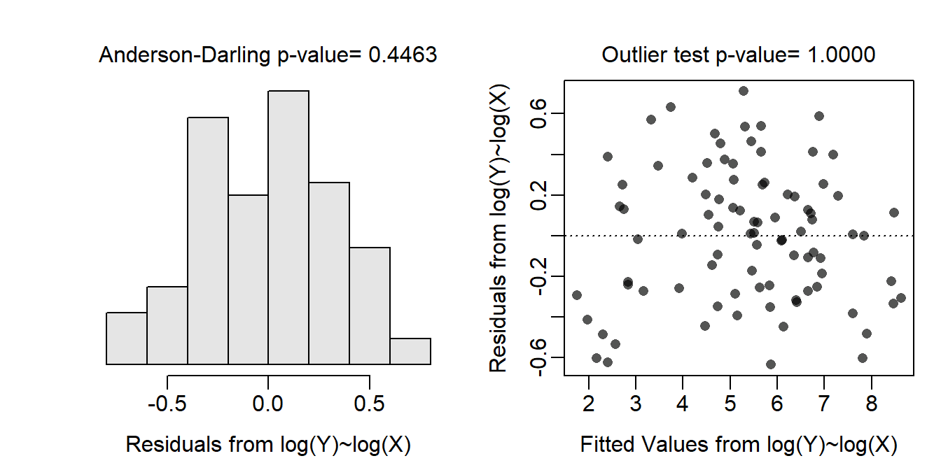
Figure 19.4: Histogram of residuals (Left) and residual plot (Right) for a simple linear regression of log above ground biomass on log diameter at breast height for trees from the Miombo Woodlands.

 

The log above ground biomass and log diameter at breast height appear to be significantly related (p<0.00005; Table 19.3). In fact, 96.3% of the variability in the log above ground biomass is explained by knowing the value of the log diameter at breast height.

 

Table 19.3: ANOVA table for simple linear regression of log above ground biomass on log diameter at breast height for trees from the Miombo Woodlands.

	Df	Sum Sq	Mean Sq	F value	Pr(>F)
logDBH	1	244.86	244.86	2238.21	0
Residuals	86	9.41	0.11

 

It appears that as as the log diameter at breast height increases by 1 unit then the mean log above ground biomass increases by between 2.17 and 2.37 units (Table 19.4; Figure 19.5). More importantly, as the diameter at breast height increases by a multiple of 2.718 the mean above ground biomass increases by a multiple of between 8.80 and 10.65.

 

Table 19.4: Intercept and slope, along with 95% confidence intervals, for simple linear regression of log above ground biomass on log diameter at breast height for trees from the Miombo Woodlands.

	Est	2.5 %	97.5 %
(Intercept)	-1.94	-2.26	-1.63
logDBH	2.27	2.17	2.37

 

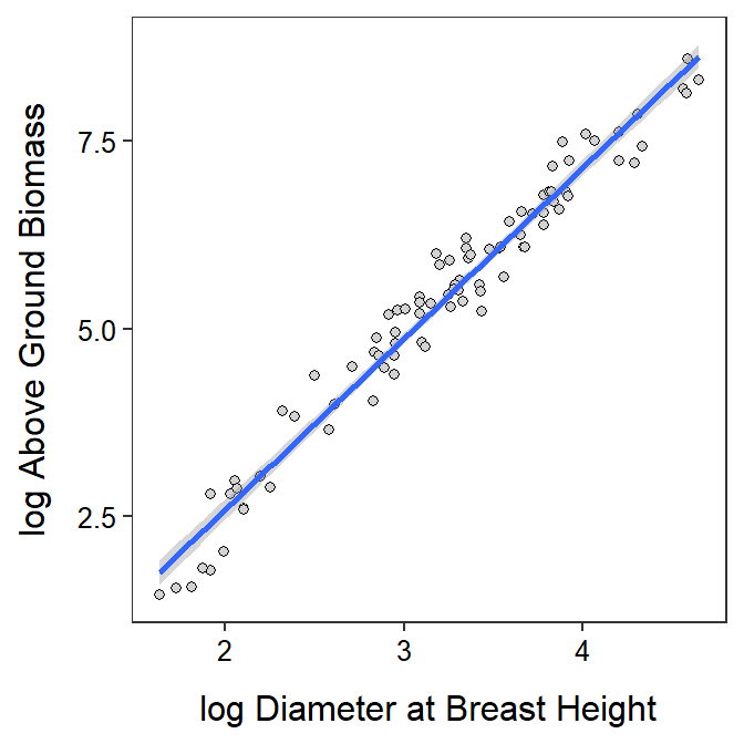
Figure 19.5: Scatterplot of log above ground biomass on log diameter at breast height for trees from the Miombo Woodlands. with the best-fit line and 95% confidence band superimposed.

 

Finally, the predicted above ground biomass for a tree with a diameter at breast height of 50 cm is between 529.9 and 2002.1 kg.

In conclusion, a significantly positive and very strong relationship was found between the natural log above-ground biomass and the natural log diameter-at-breast-height for trees in the Miombo Woodlands. A model was developed from this relationship that can be used to predict above-ground biomass of a tree from the measured DBH of the tree.

R Code and Results

tm <- read.csv("https://raw.githubusercontent.com/droglenc/NCData/master/TreesMiombo.csv")
tm <- filterD(tm,!outlier)   ## data entry error removed
lm.tm1 <- lm(AGB~DBH,data=tm)
assumptionCheck(lm.tm1)

assumptionCheck(lm.tm1,lambday=0,lambdax=0)

tm$logDBH <- log(tm$DBH)
tm$logAGB <- log(tm$AGB)
lm.tm2 <- lm(logAGB~logDBH,data=tm)
anova(lm.tm2)
rSquared(lm.tm2)
ggplot(data=tm,mapping=aes(x=logDBH,y=logAGB)) + 
  geom_point(pch=21,color="black",fill="lightgray") + 
  labs(x="log Diameter at Breast Height",y="log Above Ground Biomass") + 
  theme_NCStats() + 
  geom_smooth(method="lm")

( cfs.tm2 <- cbind(Est=coef(lm.tm2),confint(lm.tm2)) )
exp(cfs.tm2)
nd <- data.frame(logDBH=log(50))
( pl50 <- predict(lm.tm2,newdata=nd,interval="prediction") )
exp(pl50)