Module 16 SLR Models
As with all linear models, the important hypothesis tests of SLR can be reduced to comparing the lackw-of-fit for two competing models. The description below relies heavily on your previous understanding of full and simple models (see Modules 3 and 4).
16.1 Models
The full model in SLR is the equation of the best-fit line modified with an error term to represent individuals; i.e.,
\[ Y_{i} = \alpha + \beta X_{i} + \epsilon_{i} \]
where \(i\) is an index for individuals. The simple model corresponds to \(H_{0}:\beta=0\) and is thus
\[ Y_{i} = \alpha + \epsilon_{i} \]
Furthermore, it can be shown algebraically that the \(\alpha\) in the simple model is \(\mu_{Y}\).80
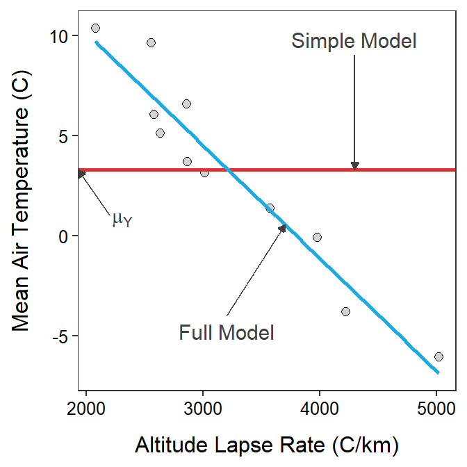
Figure 16.1: Scatterplot illustrating two competing models for describing the relationship between actual mean temperature and altitude lapse rate for Mount Everest in the winter. The horizontal red line is placed at the mean actual mean air temperatures and represents the simple model, whereas the blue line is the best-fit line and represents the full model.
Comparing Figure 16.1 to Figure 15.3 reveals that testing the simple versus the full model is the same as testing that the slope is equal to zero or not. In other words, testing for a relationship between \(Y\) and \(X\) is the same as testing that the mean value of \(Y\) is the same for all \(X\)s (i.e., simple model with no slope) or whether the mean value of \(Y\) depends on the value of \(X\) (i.e., full model with a slope).
The simple model in SLR represents a flat line at the mean of the response variable. The full model in SLR represents a line with a significant slope.
Determining whether the simple or full model should be used in SLR is a test of whether the two variables are statistically related.
16.2 ANOVA Table
Of course, the lack-of-fit of a model is measured by summing the squared residuals using predictions from the model. The lack-of-fit of the simple model is calculated with residuals from the mean value of the response variable (Figure 16.2-Left) or
\[ \text{SS}_{\text{Total}} = \sum_{i=1}^{n}\left(y_{i}-\overline{Y}_{\cdot}\right)^{2} \]
This calculation is exactly the same as that discussed for the one- and two-way ANOVAs. The lack-of-fit of the full model is calculated with residuals from the best-fit regression line (Figure 16.2-Center) or
\[ \text{SS}_{\text{Residual}} = \sum_{i=1}^{n}\left(y_{i}-\hat{\mu}_{Y|X}\right)^{2} = \sum_{i=1}^{n}\left(y_{i}-\left(\hat{\alpha}+\hat{\beta}x_{i}\right)\right)^{2} \]
This is termed SSResidual in SLR, but it is exactly analogous to SSWithin from Modules 5 and (ANOVA2Foundations2).
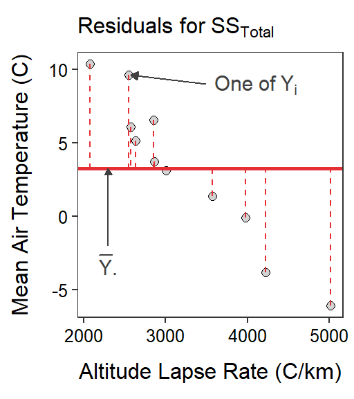
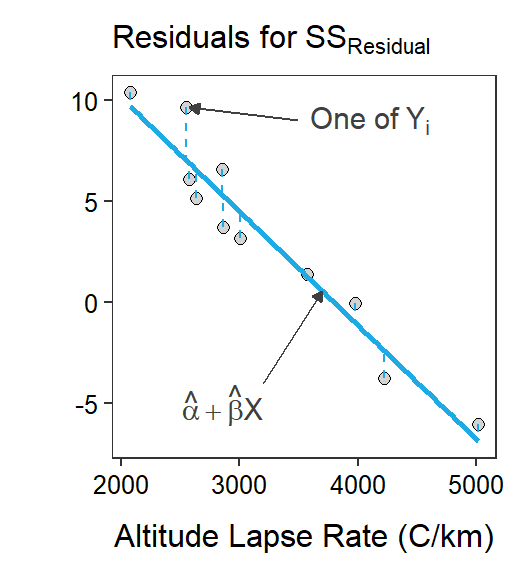
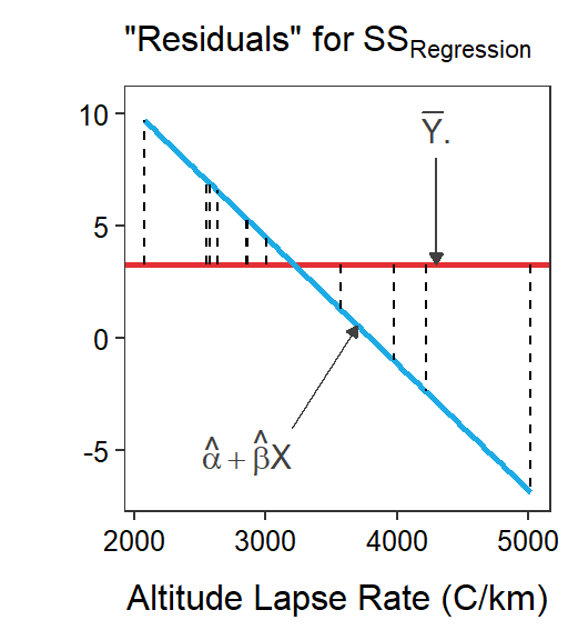
Figure 16.2: Scatterplots illustrating two competing models for describing the relationship between actual mean air temperature and altitude lapse rate for Mount Everest in winter. The horizontal red line is placed at the mean actual mean air temperature and represents the simple model. The blue line is the best-fit line and represents the full model. Residuals for each model are shown on the respective graphs.
SSTotal measures the lack-of=fit of the simplest model, which is just the mean of the response variable. Thus, SSTotal measures the maximum lack-of-fit of any model to the response variable.
As always, SSTotal partitions into two parts, labeled here as SSResidual and SSRegression. As stated above SSResidual is exactly analogous to SSWithin. Similarly SSRegression is exactly analogous to SSAmong. Thus, SSRegression measures the reduction in lack-of-fit from using the full model over the simple model (i.e., how much better the full model fits) and will become a measure of the “signal” in the data. Specifically, SSRegression is calculated from the difference in predictions from the full and simple models (Figure 16.2-Right); i.e.,
\[\text{SS}_{\text{Regression}} = \sum_{i=1}^{n}\left((\hat{\alpha}+\hat{\beta}x_{i})-\overline{Y}\right)^{2}\]
The df are similar to those discussed for a One-Way and Two-Way ANOVA. The dfTotal are \(n-1\) because there is only one parameter in the simple model. The dfResidual is \(n-2\) because the full model has two parameters (i.e., \(\alpha\) and \(\beta\)). The dfTotal partitions as before which leaves dfRegression=1, which is the difference in parameters between the full and simple models. As you can see, dfRegression is exactly analogous to dfAmong.
dfRegression is always 1 in SLR.
Per usual, MS are calculated by dividing SS by their respective df. As with the other models MSTotal=\(s_{Y}^{2}\), the total natural variability of observations (around the simple model of a single mean). The MSResidual is \(s_{Y|X}^{2}\), the natural variability of observations around the best-fit line (i.e., the full model; see Section 15.1). Finally, MSRegression is a measure of the variability of the best-fit line around the simple mean.
The F test statistic is computed as a ratio of the variance explained by the full model (i.e., the “signal”) to the variance unexplained by the full model (i.e., the “noise”) as described in Section 4.6. In SLR, this translates to
\[ F = \frac{MS_{Regression}}{MS_{Residual}} \]
which will have dfRegression numerator and dfResidual denominator df. Once again, this is exactly analogous to what we did with the One- and Two-Way ANOVAs.
The SS, MS, df, F, and p-value just discussed are summarized in an ANOVA table. Even though this is called an ANOVA table, the method is still a Simple Linear Regression. The ANOVA table is simply a common way to summarize the calculations needed to compare two models, whether those models are part of the One-Way ANOVA, Two-Way ANOVA, or Simple Linear Regression methods.
The ANOVA table for the Mount Everest air temperature and altitude lapse rate analysis is in Table 16.1. These results indicate that there is a significant relationship between the actual mean air temperature and the altitude lapse rate at stations on Mount Everest in the Winter (p<0.00005). This same result indicates that a full model with a slope term is significantly “better” at fitting the observed data then a simple model that does not contain a slope term.
| Df | Sum Sq | Mean Sq | F value | Pr(>F) | |
|---|---|---|---|---|---|
| Altitude | 1 | 245.934 | 245.934 | 115.096 | 2e-06 |
| Residuals | 9 | 19.231 | 2.137 |
In addition to the primary objective of comparing the full and simple models, several items of interest can be identified from the ANOVA table in Table 16.1.
- The variance of individuals around the regression line (\(s_{Y|X}^{2}\)) is MSResidual = 2.137.
- The variance of individuals around the overall mean (\(s_{Y}^{2}\)) is MSTotal = 26.516 (=\(\frac{245.934+19.231}{1+9}\) = \(\frac{265.165}{10}\)).
- The F test statistic is equal to the square of the t test statistic from testing \(H_{0}:\beta =0\) (see results from
summary()in Section 15.4).81
The ANOVA table for a SLR is obtained by submitting the saved lm() object to anova(). For example, Table 16.1 was obtained with anova(lm1.ev).
Note also that the F-ratio test statistic, dfRegression, dfResidual, and the p-value from the ANOVA table are shown on the last line of the output from summary(), which was introduced in Section 14.3. Also, as noted before, MSResidual is the square of the value following “Residual standard error:” in the summary() output. Thus, many of the key components of the ANOVA table are also in the summary() results.
summary(lm1.ev)#R> Coefficients:
#R> Estimate Std. Error t value Pr(>|t|)
#R> (Intercept) 21.3888561 1.7447131 12.26 6.42e-07
#R> Altitude -0.0056341 0.0005252 -10.73 1.99e-06
#R>
#R> Residual standard error: 1.462 on 9 degrees of freedom
#R> Multiple R-squared: 0.9275, Adjusted R-squared: 0.9194
#R> F-statistic: 115.1 on 1 and 9 DF, p-value: 1.987e-06
16.3 Coefficient Of Determination
The coefficient of determination (\(r^{2}\)) was introduced in Section 14.3 as a measure of the proportion of the total variability in the response variable that is explained by knowing the value of the explanatory variable. This value is actually calculated with
\[ r^{2} = \frac{SS_{Regression}}{SS_{Total}} \]
Note also that the coeffcient of determination is found in the summary() results shown above behind the “Multiple R-squared:” label.
By substituting the formula for the intercept (\(\alpha=\mu_{Y} - \hat{\beta}\mu_{X}\)) into \(\mu_{Y|X} = \alpha + \beta X\), an alternative form of the equation of the line is \(\mu_{Y|X} =\mu_{Y}+\beta\left(X-\mu_{X}\right)\). Thus, if \(\beta=0\) as in \(H_{0}\) then the simple model in \(H_{0}\) reduces to \(\mu_{Y|X}=\mu_{Y}\).↩︎
This is a general rule between the t and F distributions. An F with \(1\) numerator df and \(\nu\) denominator df is equal to the square of a t with \(\nu\) df.↩︎