Module 17 SLR Assumptions
Simple linear regressions requires five assumptions be met so that the calculations made in Modules 14-16 mean what we said they would mean. The five assumptions for a SLR are:
- independence of individuals,
- the variances of \(Y\) at each given value of \(X\) are equal (“homoscedasticity” assumption).
- the values of \(Y\) at each given value of \(X\) are normally distributed (“normality” assumption)
- no outliers or influential points, and
- the mean values of \(Y\) at each given value of \(X\) fall on a straight line (“linearity” assumption).
The first four assumptions are the same as for the One- and Two-Way ANOVAs, though they manifest slightly different in SLR. Each of these assumptions is discussed in more detail below. However, the concept of a residual plot is introduced first, as it is the primarily tool for assessing whether the SLR assumptions have been met or not.
17.1 Residual Plot
For any given best-fit line, the predicted values of \(Y\) for each observed value of \(X\) is obtained by plugging each \(X\) into the equation of the line. Predicted values are relatively “large” where the line is highest and relatively “small” where the line is lowest relative to the y-axis. A residual is computed for each value of \(X\) as well by subtracting the predicted value of \(Y\) from the observed value of \(Y\). Observations near the best-fit line have relatively “small” residuals, those far from the best-fit line have relatively “large” residuals. In addition, observations above the line have positive residuals whereas those below the line have negative residuals.82
A residual plot is a scatterplot of these residuals on the y-axis and the predicted values on the x-axis. The residual plot “transforms” the scatterplot by first “flattening” the best-fit line and placing it at 0 on the y-axis and then expanding the y-axis to remove any “dead” white space in the plot. This “transformation” effectively zooms in on the best-fit line so that you can better see how the points relate to the line.
Figure 17.1 shows a scatterplot with the best-fit line on the left and the corresponding residual plot on the right. Four points are shown to help understand how the two plots are related. This example is fairly straightforward as the residual plot essentially flattens the best-fit line and then zooms in the y-axis scale.
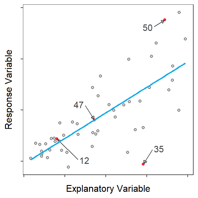
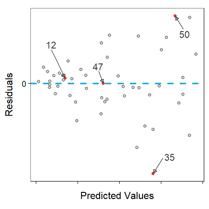
Figure 17.1: Scatterplot with best-fit line and four points highlighted (Left) and residual plot with same four points highlighted (Right).
Figure 17.2 is arranged similarly to Figure 17.1. However, in this case the scatterplot exhibits a negative relationship which makes the “transformation” to the residual plot not as obvious. With a negative relationship, the “largest” predicted values correspond to points on the left side of the scatterplot, but they end up on the right side of the residual plot. Of course, vice-versa is also true. This is most obvious with the 38th and 39th points in Figure 17.2.
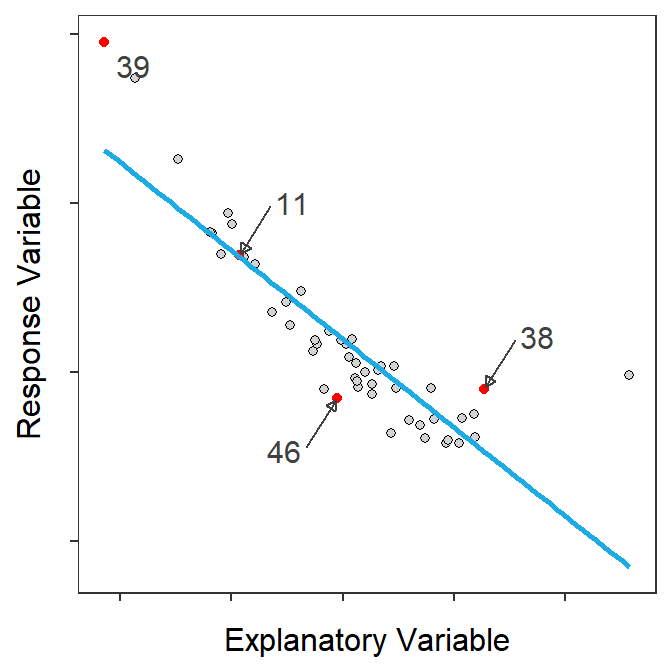
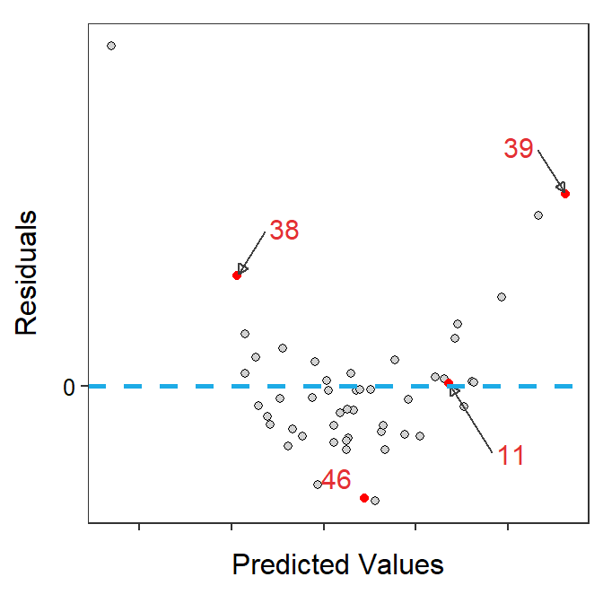
Figure 17.2: Scatterplot with best-fit line and four points highlighted (Left) and residual plot with same four points highlighted (Right).
Residual plots are like putting the scatterplot with the best-fit line under a microscope; i.e., they “zoom in” on the best-fit line to help identify how the points are arranged relative to the line.
If the homoscedasticity and linear assumptions (discussed below) are adequately met then the residual plot should exhibit no discernible or obvious pattern. Most importantly no curve nor cone or funnel-shape should be evident in the plot. Figure 17.3 is an example of a residual plot where the homoscedasticity and linearity assumptions HAVE been adequately met.
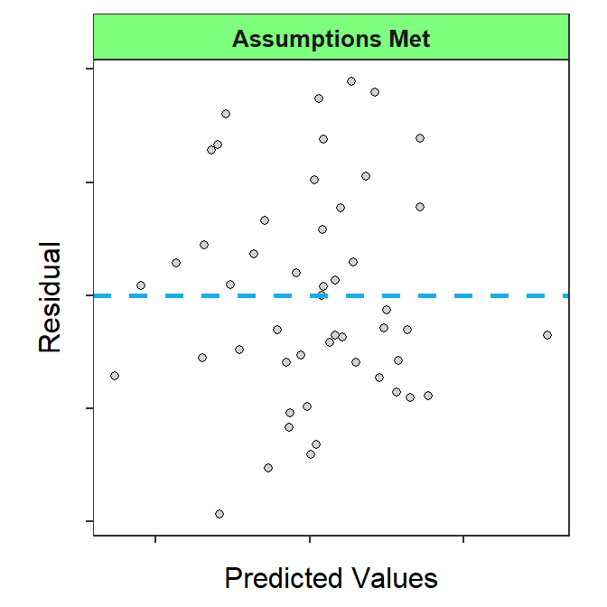
Figure 17.3: Residual plot where the homoscedasticity and linearity assumptions HAVE been adequately met.
A residual plot that exhibits no discernible or obvious patterns suggests that the homoscedasticity and linearity assumptions have been met. No pattern on a residual plot is a good thing!!
17.2 Independence
The independence assumption is largely the same as it was for a One- and Two-Way ANOVA, except that there is no need to compare within and among groups as there are no groups in an SLR. Thus, in an SLR, you need to ascertain whether individuals are independent of each other or not. This is accomplished by considering the sampling design as you did before. Individuals that are dependent are usually connected in space or time with the most common dependency occurring when multiple measurements are made on the same individuals.83
17.3 Homoscedasticity
Strictly speaking “homoscedasticity” means that the the variances of \(Y\) at each given value of \(X\) are equal. Seldom are there enough observations at the same value of \(X\) to test this assumption explicitly. Thus, in practice, homoscedasticity translates into assessing whether the same general variance or scatter of points around the line exists for all values of \(X\). Heteroscedasticity, or non-constant variance around the line, will generally appear as a cone or funnel shape on a residual plot (Figure 17.4). Sometimes the funnel-shape may be difficult to see if the linearity assumption is also not met (Figure 17.4-Right). Make sure to compare these residual plots to Figure 17.3.
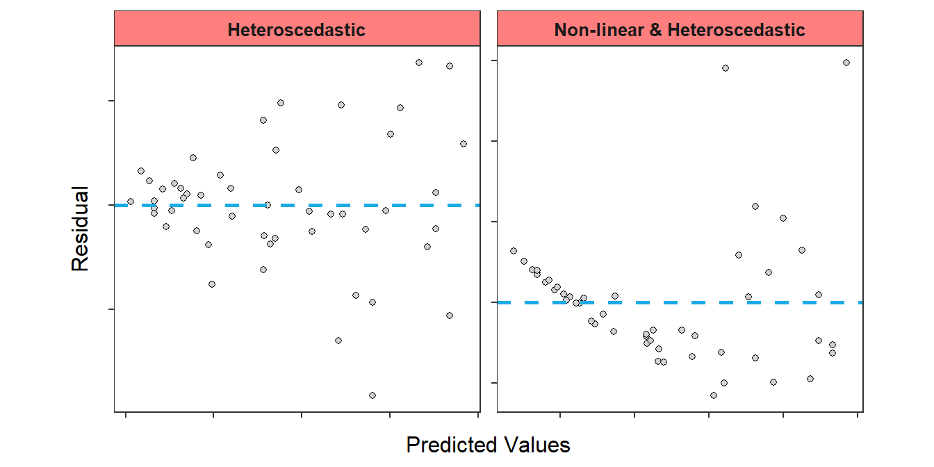
Figure 17.4: Residual plot where the homoscedasticity assumption has NOT been adequately met.
17.4 Normality
The normality assumption for SLR is assessed exactly as it was for a One- and Two-Way ANOVA; i.e., with an Anderson-Darling test and a histogram of residuals (see Section 7.3).
17.5 No Outliers or Influential Points
The no outliers assumption for SLR is assessed exactly as it was for a One- and Two-Way ANOVA; i.e., with an outlier test and a histogram of residuals (see Section 7.4).
In SLR, some individuals may be considered influential points that draw the best-fit line towards them. Some very highly influential points may so strongly draw the line to them that the line will come very close to the point and the outlier test will not identify the point as an outlier (Figure 17.5-Left). Thus, I strongly urge you to look for “abnormal” points in your residual plots (Figure 17.5-Right) rather than relying solely on the outlier test to identify problem points.
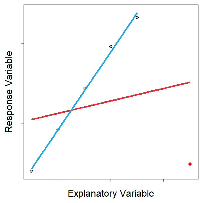
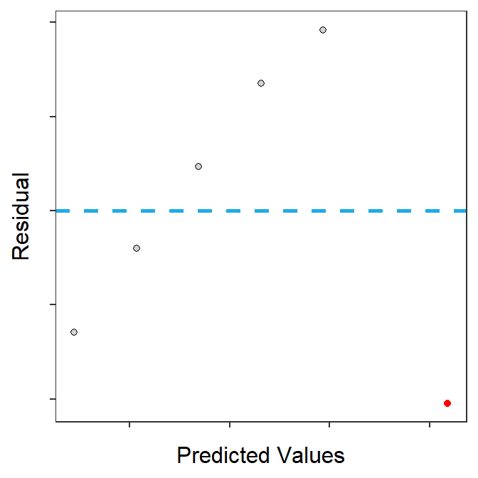
Figure 17.5: Scatterplot with a best-fit line for all points (red) and all points excluding the red point (blue) (Left) and the residual plot from the fit to all points (Right).
Influential points are a huge problem in SLR because they make the best-fit line not represent the vast majority of the data. Influential points should be removed from the data if they are clearly an error. However, if they are not an error then the SLR should be fit both with and without the point and then a narrative should be constructed that describes how the points influences the regression results.
Influential Point: An individual whose inclusion in the data set substantially impacts the coefficients of the fitted line.
17.6 Linearity
The linearity assumption is the most important assumption in SLR; i.e., the form of the bivariate relationship must be linear in order to fit a line to it! Problems with the linearity assumption are diagnosed by examination of the residual plot. The most common departures from linearity look like parabolas on the residual plot (Figure 17.6), but more “complicated” structures may also be noted. Either way, a general curve or non-linearity will be apparent in the residual plot of the linearity assumption has been violated. A non-linearity may be difficult to diagnose if the homoscedasticity assumption is also not met (Figure 17.6-Right). Make sure to compare these residual plots to Figure 17.3.
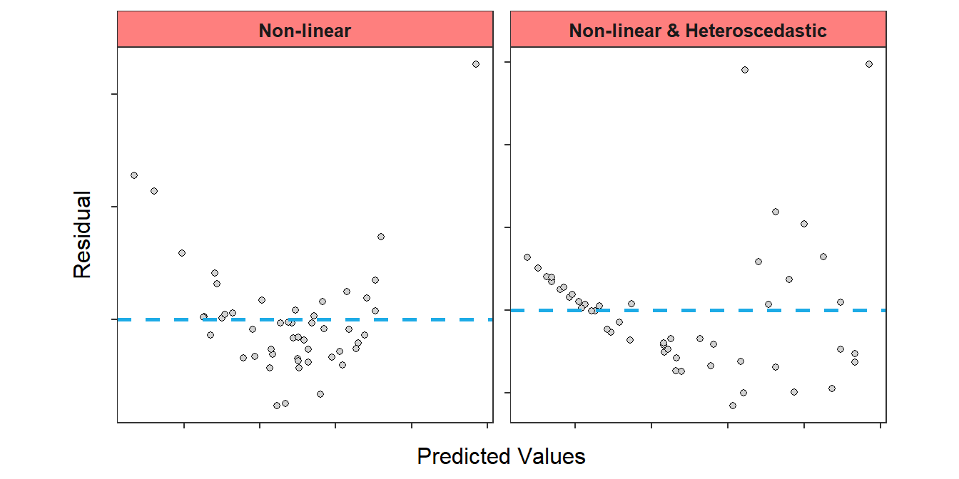
Figure 17.6: Residual plot where linearity assumption has NOT been adequately met.
17.7 Testing Assumptions in R
The residual plot, histogram of residuals, Anderson-Darling test p-value, and outlier test p-value can all be constructed by submitting the saved lm() object to assumptionCheck().84 For example, the results below indicate that all assumptions are adequately met for the Mount Everest air temperature and altitude lapse rate regression – i.e., there is no discernible or obvious curve or funnel-shape to the residual plot, the Anderson-Darling p-value indicates that the residuals are normally distributed, and the outlier test p-value does not indicate the presence of any outliers. It should be noted, however, that the sample size is very small in this case.
assumptionCheck(lm1.ev)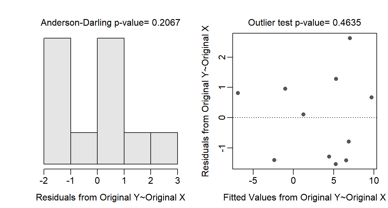
If the linearity, homoscedasticity, normality, or no outliers assumptions are not met then transformations for the response variable, explanatory variable, or both should be considered (see Module 18).
The concepts of predicted values and residuals was discussed in Module 14.↩︎
If individuals are ordered by time or space then the Durbin-Watson statistic can be used to determine if the individuals are serially correlated or not. Generally, the H0: “not serially correlated” and HA: “is serially correlated” are the hypotheses for the Durbin-Watson test. Thus, p-values <α result in the rejection of H0 and the conclusion of a lack of independence. In this case, the regression assumption would be violated and other methods, primarily time-series methods, should be considered.↩︎
This is exactly as you did for a One- and Two-Way ANOVA.↩︎