Module 20 IVR Variables
Simple linear regression is a powerful tool used to evaluate the relationship between two quantitative variables (Modules 14-19). It is common for a researcher to compare simple linear regression models fit to separate groups of individuals. Indicator variable regression (IVR),87 is a method to make these comparisons. For example, IVR methods could be used in each of the following situations.
- Determine if the relationship between propodus height and claw closing force differs among three types of crabs (Yamada and Boulding 1998).
- Determine if the proportional area covered by an invasive plant differs between sites after adjusting for different resident times for the plant (i.e., how long it has been present at a site) (Mullerova et al. 2005).
- Determine if the relationship between the sales of a product and the price of the product differs among regions of the country.
- Determine if the relationship between total body electrical conductivity and lean body mass (a method used to measure body fat) differs between live and dead birds of various species (Castro et al. 1990).
- Determine if the relationship between a pitcher’s earned run “average” (ERA) and the average pitch speed at the point of release differs among pitchers in the National and American Leagues.
As shown in each of these examples, an IVR consists of a quantitative response variable, a single quantitative explanatory variable, and a second categorical explanatory variable that identifies the groups. As is common with IVRs, the quantitative explanatory variable will be referred to as a covariate and the categorical explanatory variable will be referred to as a factor.88
Covariate: The quantitative explanatory variable in an IVR model.
In this course, we will only consider one factor, though the methods described here easily extend to multiple factors. An IVR with a single factor variable is called a one-way IVR model.
Example Data
Throughout this and the next few modules, we will refer to a study by Makarewicz et al. (2003), who examined the relationship between the concentration of mirex in the tissue and the weight of salmon.89 They collected these data on Coho Salmon (Oncorhynchus kisutch) and Chinook Salmon (Oncorhynchus tshawytscha) in six different years. They were interested in determining if the relationship between mirex and weight differed between the two species or if it differed among years (Table 20.1).
| year | weight | mirex | species |
|---|---|---|---|
| 1977 | 0.41 | 0.16 | chinook |
| 1977 | 4.77 | 0.22 | coho |
| 1982 | 2.92 | 0.22 | chinook |
| 1986 | 1.70 | 0.12 | coho |
| 1986 | 9.53 | 0.41 | chinook |
| 1996 | 0.90 | 0.07 | coho |
| 1999 | 2.61 | 0.03 | coho |
| 1999 | 11.82 | 0.09 | chinook |
20.1 Indicator Variables
Only Two Levels
An indicator variable contains numeric “codes” created from a factor variable, which are required for inclusion in a linear model. Specifically, an indicator variable consists of 0s and 1s, where a 1 indicates that the individual has a certain characteristic and a 0 indicates that it does not have the characteristic.90
For example, the species factor variable in the salmon mirex data could be converted to an indicator variable that is designed as follows:
\[ COHO = \left\{\begin{array}{l} 1 \text{ if a Coho salmon }\\ 0 \text{ if NOT a Coho salmon} \end{array} \right. \]
Alternatively, the same factor variable could be used to create the following indicator variable:
\[ CHINOOK = \left\{\begin{array}{l} 1 \text{ if a Chinook salmon }\\ 0 \text{ if NOT a Chinook salmon} \end{array} \right. \]
Importantly, both of these indicator variables would not be used as each one exhausts the possibilities. For example, if COHO=1 you know you have a Coho Salmon and if COHO=0 you know that you have a Chinook Salmon.
For consistency and ease of remembering the coding, an indicator variable should be named after the characteristic denoted by a 1. The two examples above followed this rule – the COHO indicator variable was a 1 when the fish was a Coho Salmon and the CHINOOK indicator variable was a 1 when the fish was a Chinook Salmon.
If a factor with two levels can be cast as two indicator variables, but only one of those indicator variables is needed, then which one should be used? Analytically, it does not matter as the same conclusions will be reached no matter which indicator variable you use. However, in R, factor levels are arranged alphabetically and a 0 is assigned to the first level and, thus, a 1 is assigned to the second level. Thus, R names indicator variable after the alphabetically second group. To maintain consistency with R you should follow this convention. For example, R will and we should use COHO as “Coho” comes after “Chinook.”
The relationship between the original factor variable and the indicator variable is easy to keep track of when there are only two groups, but is more work with more groups (see next section). A table with groups shown in the left-most column and the indicator variable(s) with its codes shown in the right-most column(s) will help keep track of the codings when there are more groups.
| species | COHO |
|---|---|
| chinook | 0 |
| coho | 1 |
Indicator Variable: A variable that is a numerical representation of a dichotomous (or binary or binomial) categorical variable.
Indicator variables will be coded as 0 for individuals that do NOT have the characteristic of interest and 1 for individuals that do have the characteristic of interest.
Indicator variables should be named after the “1” group so that it is easy to remember the coding scheme being used.
More than Two Levels
Combinations of indicator variables can be used to code factor variables that consist of more than two levels. For example, Makarewicz et al. (2003) were also interested in determining if the relationship between mirex concentration and weight of the salmon differed among six collection years. For simplicity and space considerations, let’s consider that they were interested in only three years – 1977, 1982, and 1986. In this simpler situation, two indicator variables would be created to represent the year factor variable. For example,
\[ YEAR1982 = \left\{\begin{array}{l} 1 \text{ if collected in 1982 }\\ 0 \text{ if NOT collected in 1982 } \end{array} \right. \]
and
\[ YEAR1986 = \left\{\begin{array}{l} 1 \text{ if collected in 1986 }\\ 0 \text{ if NOT collected in 1986} \end{array} \right. \]
Note that it is possible to create a third dummy variable to represent salmon collected in 1977. However, this indicator variable is redundant with YEAR1982 and YEAR1986 because when YEAR1982=0 and YEAR1986=0 then the salmon must have been collected in 1977. This illustrates the rule that the number of indicator variables required is one less than the number of levels to be coded.91 An example table showing the codings is below.
| year | YEAR1982 | YEAR1986 |
|---|---|---|
| 1977 | 0 | 0 |
| 1982 | 1 | 0 |
| 1986 | 0 | 1 |
The level denoted by the group with “0”s for all related indicator variables is called the reference group. In the last example above, salmon collected in 1977 would be the reference group. It will be shown in Module 21 that all comparisons of intercepts and slopes in the analysis will “refer” to this group of individuals.
Suppose, for illustration purposes, that you wanted fish collected in 1982 to be the reference group. In this situation, YEAR1982 would be replaced with YEAR1977 and the table relating the year factor variable to the indicator variables would be as shown below.
| year | YEAR1977 | YEAR1986 |
|---|---|---|
| 1977 | 1 | 0 |
| 1982 | 0 | 0 |
| 1986 | 0 | 1 |
One less indicator variable is needed then the number of categories in the factor variable.
Reference group: The category or group that is represented by zeroes for all indicator variables.
Changing the reference group in an analysis requires changing the indicator variables used in the analysis.
20.2 Interaction Variables
An interaction variable is an explanatory variable that is the product of two or more other explanatory variables (see Module 10). In IVR models, interaction variables are created between the covariate and each of the indicator variables. Thus, there will always be as many interaction variables as there are indicator variables in an IVR. For example, in the example with Coho and Chinook Salmon, there would be one interaction variable – COHO:Weight. However, in the the example with the three years of data there would be two interaction variables – YEAR1982:Weight and YEAR1986:Weight.
Interaction variables serve the same purpose in an IVR as they did in a Two-Way ANOVA (see Module 10). That is, the interaction variable is used to identify if the effect of one explanatory variable (here the covariate) on the response variable differs depending on the other explanatory variable (here the factor). In other words, an interaction variable will be used to determine if the effect of the covariate on the response variable differs among groups (i.e., levels of the factor). For example, the interaction variable will be used to determine if the effect of weight of the salmon on the concentration of mirex in the tissue differs by species of salmon.
The interaction between two variables in an IVR model is illustrated with the examples in Figure 20.1. In the left panel, the effect of salmon weight (the covariate) on mirex concentration in the tissue (the response) is the same for Coho and Chinook Salmon. This is illustrated by each species having the same slope.92 However, different slopes in the right panel indicate that the effect of salmon weight on mirex concentration in the tissue differs between the two species. In this particular example, the relationship is “flatter” for Coho than for Chinook Salmon. Thus, an interaction exists for the situation depicted in Figure 20.1-Right, because the effect of the covariate on the response depends on which group is being considered. Graphically, an interaction is illustrated by non-parallel lines.
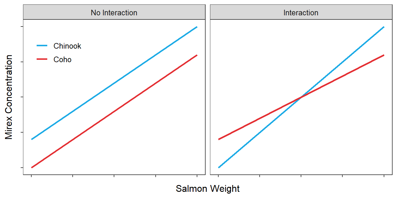
Figure 20.1: Idealized fitted-line plots representing an IVR fit to two groups. The graph on the left indicates the absence of an interaction. The graph on the right indicates the presence of an interaction.
Interaction variables in IVR are constructed from the covariate and each indicator variable. Thus, there are as many interaction as indicator variables in an IVR.
Interaction variables in IVR are used to determine if the effect of the covariate on the response variable differs among groups defined by the indicator variable(s).
Parallel lines indicate no interaction effect; non-parallel lines indicate an interaction effect.
This is not a standard name. Some authors call it dummy variable regression (e.g., Fox 1997), whereas others call it Analysis of Covariance (ANCOVA). I will not use either of these terms as I prefer the word “indicator” to “dummy” and I will reserve the ANCOVA method for the situation where the separate SLR models are known or assumed to have equal slopes. Thus, ANCOVA models are a subset of the IVR models discussed here. It should also be noted that some authors (e.g., Weisberg 2005) do not use a separate name for IVR but simply include it as a multiple linear regression model.↩︎
Similar to what was one with the One- and Two-Way ANOVAS in Modules 5-13.↩︎
Mirex is a chlorinated hydrocarbon that was commercialized as an insecticide. Use of mirex was banned in 1976 because of its impact on the environment.↩︎
Other coding schemes exist. For example, “contrast coding” uses -1 and 1. However, the 0 and 1 coding scheme leads to simpler interpretations and calculations and, thus, is used throughout this course.↩︎
This is only true if an intercept term exists in the regression model, which will be the case for all models in this course.↩︎
In regression the “effect” of the explanatory variable on the response variable is measured by the slope.↩︎