Module 24 IVR Summary

Specific parts of a full Indicator Variable Regression (IVR) analysis were described in Modules 20-23. In this module, a workflow for a full analysis is offered and that workflow is demonstrated with several examples.

24.1 Suggested Workflow

The following is a process for fitting an IVR. Consider this process as you learn to fit IVR models, but don’t consider this to be a concrete process for all models.

1. Briefly introduce the study (i.e., provide some background for why this study is being conducted).
2. State the hypotheses to be tested.
3. Show the sample size per group using xtabs() and comment on whether the study was balanced (i.e., same sample size per group) or not.
4. Assess the independence assumption.
   • If this assumption is not met then other analysis methods must be used.
5. Fit the untransformed ultimate full model with lm().
6. Check the other four assumptions for the untransformed model with assumptionCheck().
   • Check linearity of the relationship with the residual plot.
   • Check homoscedasticity with the residual plot.
   • Check normality of residuals with an Anderson-Darling test and histogram of residuals.
   • Check outliers and influential points with the outlier test and residual plot.
7. If an assumption or assumptions are violated, then attempt to find a transformation where the assumptions are met.
   • Use trial-and-error with assumptionCheck(), theory (e.g., power or exponential functions), or experience to identify possible transformations for the response variable and, possibly, for the explanatory variable.
     • Attempt transformations with the response variable first.
     • Generally only ever transform the explanatory variable with logarithms.
   • If only an outlier or influential observation exists (i.e., linear, homoscedastic, and normal residuals) and no transformation corrects the “problem,” then consider removing that observation from the data set.
   • Fit the ultimate full model with the transformed variable(s) or reduced data set.
8. Construct an ANOVA table for the ultimate full model with anova().
   • If a significant interaction exists then do NOT interpret the main effects!!
   • If a significant interaction does NOT exist then interpret the main effects (i.e., interpret the coincident lines and relationship test p-values).
9. As appropriate, perform multiple comparisons to identify specific differences.
   • If a significant interact exists (i.e., non-parallel lines) then use emtrends() and summary() to identify specific slopes that differ.
   • If a significant interaction does not exist (i.e., parallel lines) but the lines are not coincident (i.e., different slopes) …
     • Fit a new model without the insignificant interaction term.
     • Use emmeans() and summary() to identify specific mean values of the response at the mean value of the covariate that differ.
10. Create a summary graphic of the fitted lines using the ggplot().
    • Include the 95% confidence band and the observed data as long as the plot is not overly cluttered. If it is, just show the fitted lines.
11. Make predictions with predict(), if desired.
12. Write a succinct conclusion of your findings. Make sure you address …
    • whether the relationship between the response variable and the covariate differs among groups.
    • whether the mean value of the response variable at the mean value of the covariate differs among groups (if appropriate to address this).
    • whether there is a significant relationship between the response variable and the covariate (may need to do separately for each group).

 

24.2 Fish Energy Density (No Transformation)

Some ecologists study the transfer of energy through the ecosystem. Energy is passed up trophic levels through predation. How much energy is transferred depends on a number of things, including the energy density of the prey. Hartman and Brandt (1995) provided a meta-analysis of energy densities for a wide variety of prey fishes. In one part of that study they more closely examined the energy densities of Bay Anchovy (Anchoa mitchilli), Bluefish (Pomatomus saltatrix), Striped Bass (Morone saxatilis), and Weakfish (Cynoscion regalis) collected from Chesapeake Bay , Maryland.

Hartman and Brandt (1995) were primarily interested in describing differences in energy density between the four species. However, it is commonly known that the amount of energy in a fish is partly dependent on the percent dry weight of the fish.¹⁰⁵ Thus, their objectives were to (i) describe the relationship between energy density and dry weight and determine if that relationship differed among the four species and (ii) determine if the mean energy density at a constant dry weight differed among the four species.

The first hypothesis to be tested (i.e, parallel lines test) is

\[ \begin{split} \text{H}_{\text{0}}&: ``\text{the relationship between energy density and dry weight does not differ by species''} \\ \text{H}_{\text{A}}&: ``\text{the relationship between energy density and dry weight does differ by species''} \\ \end{split} \]

If this H₀ is not rejected (i.e., the lines are parallel) then the following two sets of hypotheses will be tested (i.e., coincident lines and relationship tests),

\[ \begin{split} \text{H}_{\text{0}}&: ``\text{the mean energy density at the mean dry weight does not differ among species''} \\ \text{H}_{\text{A}}&: ``\text{the mean energy density at the mean dry weight does differ among species''} \\ \end{split} \]

and

\[ \begin{split} \text{H}_{\text{0}}&: ``\text{there is not a relationship between energy density and dry weight''} \\ \text{H}_{\text{A}}&: ``\text{there is a relationship between energy density and dry weight''} \\ \end{split} \]

The sample size is quite unbalanced, with essentially twice as many Bay Anchovy as any other species (Table 24.1). The sample size for Bluefish, Striped Bass, and Weakfish is quite small.

 

Table 24.1: Sample size for each species.

species	Freq
bayanchovy	26
bluefish	13
stripedbass	14
weakfish	11

 

There is very little information to fully assess independence. However, as long as any individual fish does not affect the dry weight or the energy density of any other fish, than the independence assumption is likely met. It is hard to imagine how any one fish could affect any other single fish for these two metrics, so I suspect that independence is adequately met.

The residual plot (Figure 24.1-Right) does not exhibit any curvature or funneling pattern; thus the linearity and homoscedasticity assumptions are met. The residuals appear approximately normal (Anderson-Darling p=0.4549; Figure 24.1-Left) and no outliers are present (outlier test p>1). No transformation is needed as all assumptions appear to be met.

 

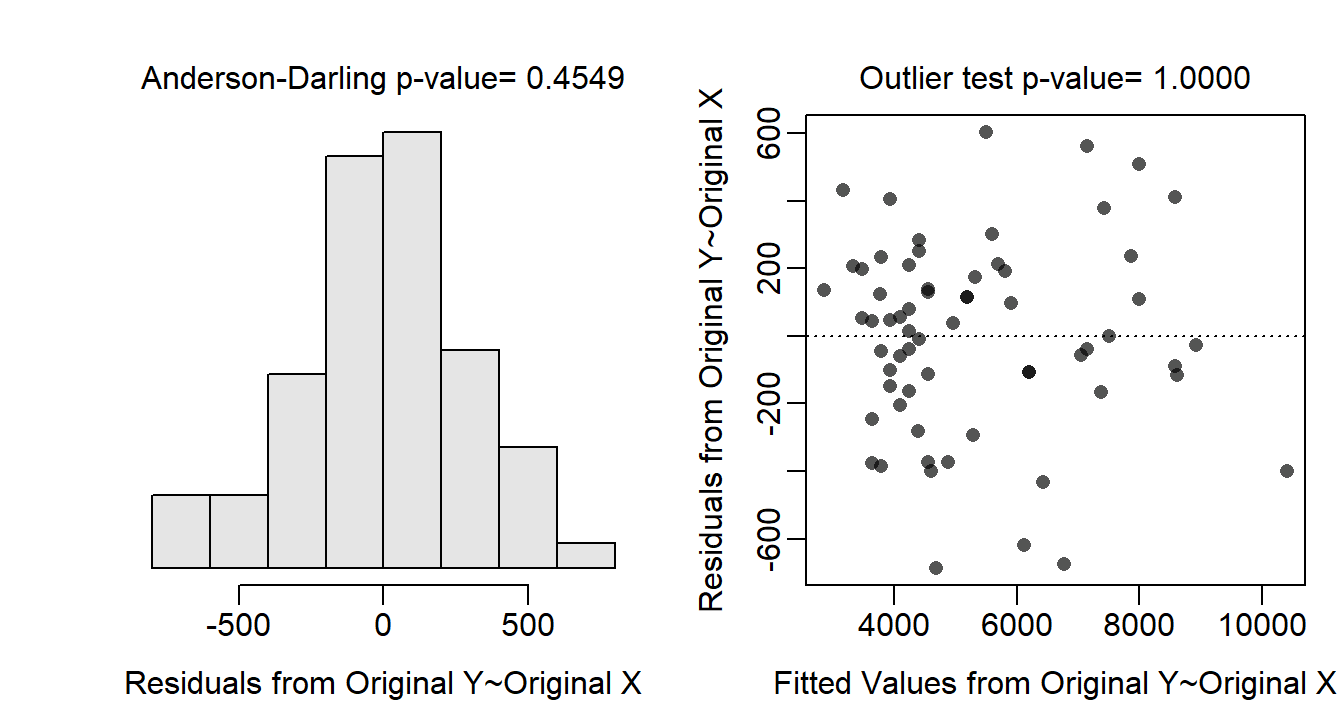
Figure 24.1: Histogram of residuals (left) and residual plot (right) for the IVR analysis of energy density by percent dry weight and species.

 

The relationship between energy density and percent dry weight differed among some of the species (p<0.00005; Table 24.2). It appears that the slope for Bay Anchovy is less than the slope for all other species (p≤0.0002; Table 24.3). The slopes do not differ among the other three species (p≥0.1444; Table 24.3).

 

Table 24.2: ANOVA table for the IVR analysis of energy density by percent dry weight and species.

	Df	Sum Sq	Mean Sq	F value	Pr(>F)
dw	1	170693154	170693154	1859.0	0e+00
species	3	10592036	3530679	38.5	0e+00
dw:species	3	4105617	1368539	14.9	3e-07
Residuals	56	5142008	91822

 

Table 24.3: Tukey’s multiple comparisons for all pairs of slopes for the IVR analysis of energy density by percent dry weight and species.

contrast	estimate	lower.CL	upper.CL	p.value
bayanchovy - bluefish	-208.3	-291.2	-125.5	0.0000
bayanchovy - stripedbass	-157.6	-241.3	-73.9	0.0000
bayanchovy - weakfish	-149.6	-237.4	-61.8	0.0002
bluefish - stripedbass	50.7	-15.9	117.3	0.1948
bluefish - weakfish	58.7	-12.9	130.4	0.1444
stripedbass - weakfish	8.0	-64.6	80.6	0.9912

 

As only Bay Anchovy had a different slope, I removed this species so that I could determine how the mean energy density at the mean percent dry weight differed among the the other three species. Assuming parallel lines for these three species (from the analysis above), it appears that the intercepts differed among some of the species (p=0.0005; Table 24.4). Tukey’s multiple comparisons indicate that the intercept for Bluefish is less than the intercept for both Striped Bass and Weakfish (p≤0.0178; Table 24.5). The intercepts for Striped Bass and Weakfish did not differ (p=0.7088; Table 24.5).

 

Table 24.4: ANOVA table for the IVR analysis of energy density by percent dry weight and species with Bay Anchovy excluded and assuming parallel lines (from the previous analysis).

	Df	Sum Sq	Mean Sq	F value	Pr(>F)
dw	1	104962559	104962559	782.4	0.00000
species	2	2583571	1291785	9.6	0.00049
Residuals	34	4561501	134162

 

Table 24.5: Tukey’s multiple comparisons for all pairs of mean energy density at the mean percent dry weight by species.

contrast	estimate	lower.CL	upper.CL	p.value
bluefish - stripedbass	-631.4	-988.4	-274.4	0.0004
bluefish - weakfish	-506.5	-935.9	-77.1	0.0178
stripedbass - weakfish	124.9	-260.3	510.2	0.7088

 

Through this analysis it appears that Bay Anchovy has a less steep relationship between energy density and percent dry weight than the other species (Figure 24.2). So, energy density does not increase as quickly with increasing dry weight for Bay Anchovy as it does for the other species. Among the other species, it appears that Bluefish has a lower mean energy density at all percent dry weights than Striped Bass and Weakfish. Striped Bass and Weakfish appear to have the same mean energy density at all percent dry weights. Thus, for fish of the same percent dry weight, Striped Bass and Weakfish have a higher mean energy density than Bluefish.

 

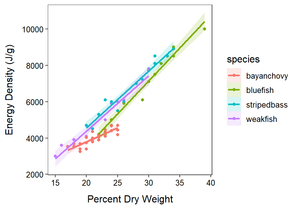
Figure 24.2: Fitted lines for the regression of energy density on percent dry weight separated by species of fish.

 

R Code and Results

nrg <- read.csv("http://derekogle.com/Book207/data/FishEnergyDensity.csv")
xtabs(~species,data=nrg)
ivr1.nrg <- lm(ed~dw+species+dw:species,data=nrg)
assumptionCheck(ivr1.nrg)

anova(ivr1.nrg)
mc1.nrg <- emtrends(ivr1.nrg,specs=pairwise~species,var="dw")
( mc1sum.nrg <- summary(mc1.nrg,infer=TRUE) )
nrg2 <- filter(nrg,species!="bayanchovy")
ivr2.nrg <- lm(ed~dw+species,data=nrg2)
anova(ivr2.nrg)
mc2.nrg <- emmeans(ivr2.nrg,specs=pairwise~species)
( mc2sum.nrg <- summary(mc2.nrg,infer=TRUE) )
ggplot(data=nrg,mapping=aes(x=dw,y=ed,color=species,fill=species)) + 
  geom_point() + 
  labs(x="Percent Dry Weight",y="Energy Density (J/g)") + 
  theme_NCStats() + 
  geom_smooth(method="lm",alpha=0.15)

 

24.3 Shrub Allometry (Transformation)

Allometric models are useful for assessing above-ground biomass (AGB) and net primary productivity (ANPP) of forests and shrubs. These models are widely used for forest inventory and management because they offer a non-destructive, relatively accurate, and labor-efficient method for estimating these difficult to measure metrics. The AGB and ANPP of plants are important components of the global carbon cycle. Above-ground biomass can be used to quantify carbon stores in plants and ANPP can help to understand potential future carbon storage. Thus, the prediction of AGB and ANPP of plants will help to evaluate terrestrial carbon sequestration, which is important for mitigation of global climate change.

Allometric models to be used for these purposes are developed for individual tree and shrub species, oftentimes for different habitats. She et al. (2015) examined allometric relationships for the xeric shrub Artemisia ordosica, a species endemic to the Mu Us Desert in China. In one part of their analysis they used crown area (CA; m²) and habitat type to explain variability in AGB (kg) of individual Artemisia shrubs. Three habitats were considered – semi-fixed dunes (SF), fixed dunes (FD), and fixed dunes with soil crusts (FC). All individual Artemisia plants were sampled from three plots that were 2-4 km separated. In their model fitting they assumed that the relationship between AGB and CA followed a power function, as is typical for many allometric relationships.

The first hypothesis to be tested (i.e, parallel lines test) is

\[ \begin{split} \text{H}_{\text{0}}&: ``\text{the relationship between AGB an CA does not differ by habitat''} \\ \text{H}_{\text{A}}&: ``\text{the relationship between AGB an CA does differ by habitat''} \\ \end{split} \]

If this H₀ is not rejected (i.e., the lines are parallel) then the following two sets of hypotheses will be tested (i.e., coincident lines and relationship tests),

\[ \begin{split} \text{H}_{\text{0}}&: ``\text{the mean AGB at the mean CA does not differ among habitats''} \\ \text{H}_{\text{A}}&: ``\text{the mean AGB at the mean CA does differ among habitats''} \\ \end{split} \]

and

\[ \begin{split} \text{H}_{\text{0}}&: ``\text{there is not a relationship between ABG and CA''} \\ \text{H}_{\text{A}}&: ``\text{there is a relationship between AGB and CA''} \\ \end{split} \]

The sample size is unbalanced, with essentially 50% more Artemisia sampled in semi-fixed (SF) dunes than the other two habitats (Table 24.6). The sample sizes are not large but are likely adequate in all habitats.

 

Table 24.6: Sample size of individual plants by habitat.

Habitat	Freq
FC	22
FD	23
SF	31

 

Independence of individual plants is questionable both within- and among- groups. Though the three plots were spatially separated, it appears that multiple plants were sampled in each plot. Thus, there could be an effect of one plant on another plant in the same plot. That being said, it is hard to imagine that one plant could affect the relationship between crown area and above-ground biomass of another plant in the same plot. Thus, I will tentatively continue assuming independence.

Allometric relationships often follow a power function, thus the assumptions are likely not met on the original untransformed scale. Indeed, the residual plot (Figure 24.3-Right) shows a clear curvature and heteroscedasticity. A power function relationship suggests that both the response and covariate should be log-transformed. With both variables log-transformed the residual plot (Figure 24.4-Right) exhibits no curvature or funnel-shape, which indicates that the linearity and homoscedasticity assumptions are met on this scale. The residuals are approximately normal (Anderson-Darling p=0.6638; Figure 24.4-Left) and no outliers are present (outlier test p=0.2764). The analysis will continue on the log-log scale as all assumptions appear to be met on this scale.

 

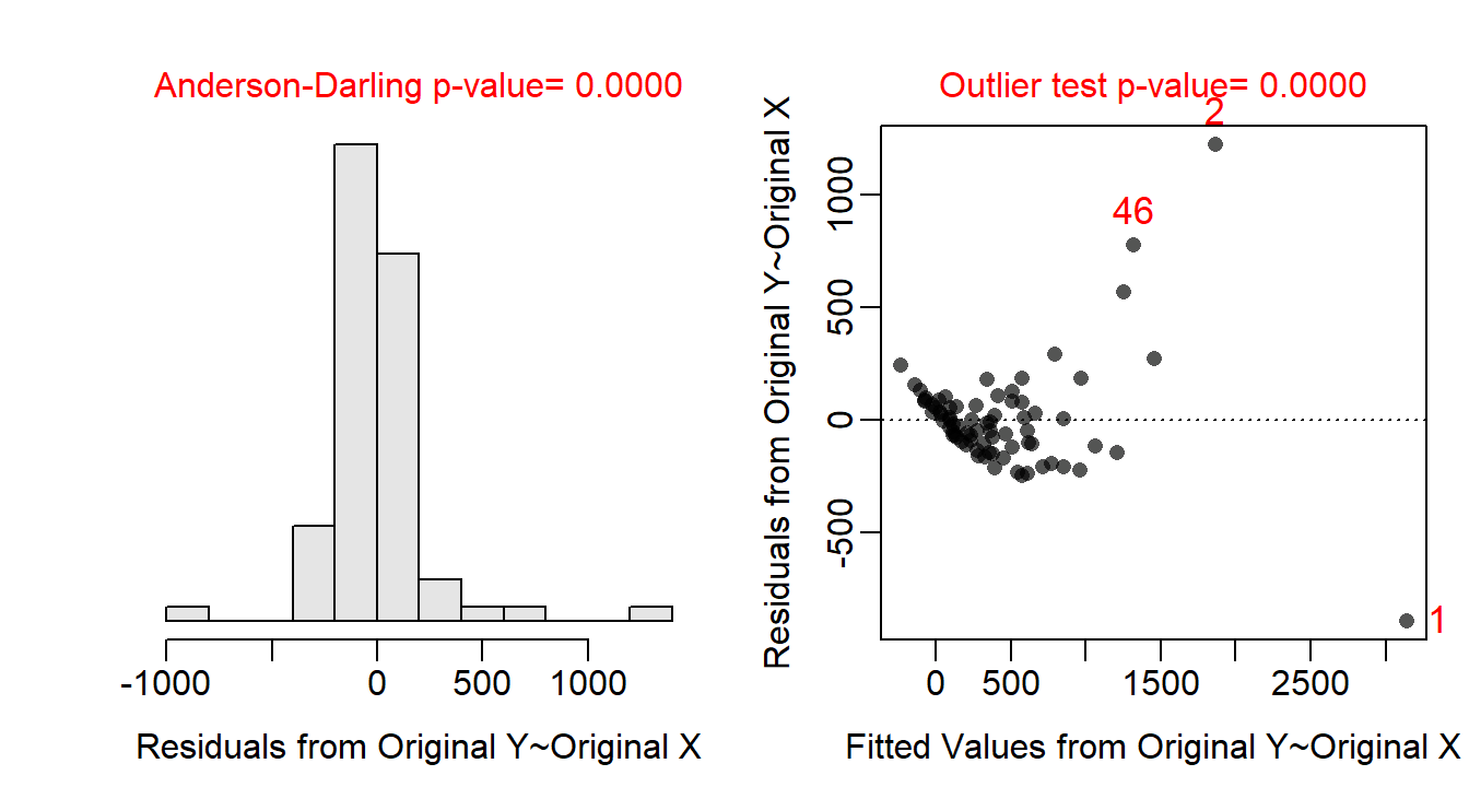
Figure 24.3: Histogram of residuals (Left) and residual plot (Right) for the IVR of above-ground biomass on crown area for three dune habitats.

 

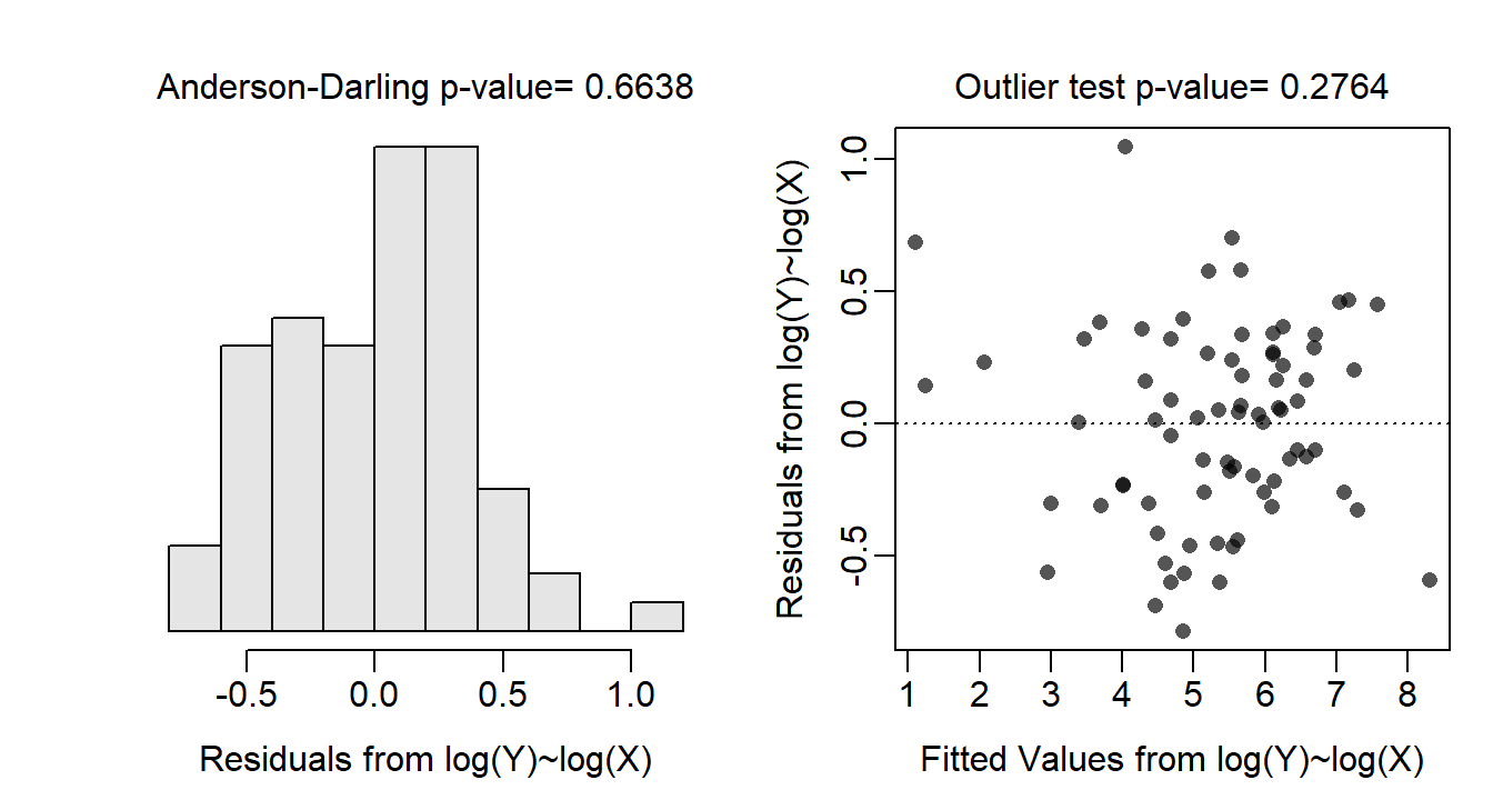
Figure 24.4: Histogram of residuals (Left) and residual plot (Right) for the IVR of log-transformed above-ground biomass on log-transformed crown area for three dune habitats.

 

The relationship between log above-ground biomass and log crown area does not differ among Artemisia sampled from the different habitats (p=0.1115; Table 24.7). There does appear to be a significant relationship between log above-ground biomass and log crown area for Artemisia (p<0.00005; Table 24.7). Finally, it appears that the mean log above-ground biomass at all log crown areas differs between some of the habitats (p<0.00005; Table 24.7).

 

Table 24.7: ANOVA table for the IVR of log-transformed above-ground biomass on log-transformed crown area for three dune habitats.

	Df	Sum Sq	Mean Sq	F value	Pr(>F)
logCA	1	120.72	120.72	826.34	0.0000
Habitat	2	13.65	6.83	46.73	0.0000
logCA:Habitat	2	0.66	0.33	2.26	0.1115
Residuals	70	10.23	0.15

 

The back-transformed mean above-ground biomass at the back-transformed mean crown area differs among all habitats (p≤0.0001; Table 24.8). The back-transformed mean above-ground biomass at the back-transformed mean crown area is between 1.350 and 2.356% greater in the soil crust (FC) than fixed dune (FD) habitats, between 2.198 and 3.737 times greater in the soil crust (FC) than semi-fixed dune (FD) habitats, and between 1.241 and 2.081 times greater in the fixed dune (FD) than semi-fixed dune habitats (Table 24.8).

 

Table 24.8: Tukey’s multiple comparisons for the RATIO mean above-ground biomass at the mean log crown areas for each pair of habitats

contrast	ratio	lower.CL	upper.CL	t.ratio
FC / FD	1.783	1.350	2.356	4.972475
FC / SF	2.866	2.198	3.737	9.497782
FD / SF	1.607	1.241	2.081	4.397433

 

A positive relationship was found between log above-ground biomass and log crown area that did not differ between habitat types (Figure 24.5). The mean above-ground biomass for plants with the same crown area was greater for Artemisia in the surface crust habitats than in the fixed dunes habitats which were greater than in the semi-fixed dunes habitats (Figure 24.6). In other words, it appears that the above-ground biomass is greater in the surface crust habitats than fixed-dunes than semi-fixed dunes for plants with the same crown area.

 

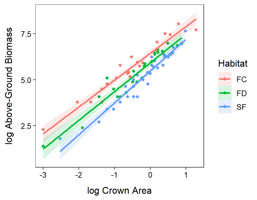
Figure 24.5: Fitted lines for the regression of log above-ground biomass on log crown area separated by habitats. Note that these lines are statistically parallel, have statistically different intercepts, and exhibit a statistically positive relationship.

 

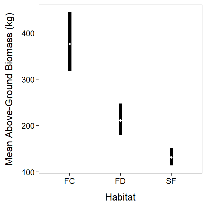
Figure 24.6: Back-transformed mean above-ground biomass of Artemisia (and 95% confidence interval) at the back-transformed mean crown area for each habitat (FC=surface crust, FC=fixed-dune, and SF=semi-fixed dune).

 

R Code and Results

shrub <- read.csv("http://derekogle.com/Book207/data/Artemisia.csv")
xtabs(~Habitat,data=shrub)
ivr1.shrub <- lm(AGB~CA+Habitat+CA:Habitat,data=shrub)
assumptionCheck(ivr1.shrub)

assumptionCheck(ivr1.shrub,lambday=0,lambdax=0)

shrub$logAGB <- log(shrub$AGB)
shrub$logCA <- log(shrub$CA)
ivr1t.shrub <- lm(logAGB~logCA+Habitat+logCA:Habitat,data=shrub)
anova(ivr1t.shrub)
ivr2t.shrub <- lm(logAGB~logCA+Habitat,data=shrub)
mc2t.shrub <- emmeans(ivr2t.shrub,specs=pairwise~Habitat,tran="log")
( mc2tsum.shrub <- summary(mc2t.shrub,infer=TRUE,type="response") )
ggplot(data=shrub,mapping=aes(x=logCA,y=logAGB,color=Habitat,fill=Habitat)) + 
  geom_point() + 
  labs(x="log Crown Area",y="log Above-Ground Biomass") + 
  theme_NCStats() + 
  geom_smooth(method="lm",alpha=0.15)

ggplot(data=mc2tsum.shrub$emmeans,
       mapping=aes(x=Habitat,y=response,ymin=lower.CL,ymax=upper.CL)) +
  geom_errorbar(size=2,width=0) +
  geom_point(pch=21,fill="white") +
  labs(y="Mean Above-Ground Biomass (kg)",x="Habitat") +
  theme_NCStats()

 

---

105. Percent dry weight is the dry weight divided by the wet weight of the fish times 100.↩︎