Module 10 Two-Way Conceptual Foundation
In contrast to a one-way ANOVA, a two-way ANOVA allows for simultaneously determining whether the mean of a quantitative response variable differs according to the levels of two grouping variables or an interaction between the two. For example, consider the following situations:
- Determining the effect of UV-B light intensity and tadpole density on mean growth of Plains Leopard Frog (Rana blairi) tadpoles (Smith et al. 2000).
- Whether mean monoterpene levels in Douglas firs (Pseudotsuga menziesii) differ depending on exposure to ambient or elevated levels of CO2 and ambient or elevated levels of temperature (Snow et al. 2003).
- Whether mean microcystin-LR concentration (a common cyanotoxin) differed by time (days) and exposure type (control (no exposure), direct exposure, or indirect exposure) to duckweed (Lemna gibba) (LeBlanc et al. 2005).
- Whether the mean rating of the “attractiveness” of a college campus differed between people who viewed a website about the campus and those that viewed the campus through GoogleMaps using a virtual-reality headset and among three different age groups of viewers (Singh et al. 2019).
The theory and application of two-way ANOVAs are discussed in this module. The presentation here depends heavily on the foundational material discussed for One-Way ANOVAs.
10.1 Two Factors
It is both possible and advantageous to manipulate more than one factor at a time to determine the effect of those factors on the response variable. For example, an experimenter may manipulate both the density of tadpoles and the level of exposure to UV-B light to determine the effect of both of these explanatory variables on body mass of tadpoles. The design of such an experiment and why it is beneficial to simultaneously manipulate two factors, as compared to varying each of those factors alone in two separate experiments, is examined in this section.
10.1.1 Design
Suppose that we are interested in the impact of two different UV-B light intensity levels (simply called “High” and “Low”) and the density of tadpoles (1, 2, and 4 individuals per tank) on the body mass (g) of tadpoles. Further suppose that we have access to 90 tanks in which to conduct this work, where each tank will be stocked with one of the tadpole densities and exposed to one of the UV-B light intensities. After a period of time the body mass of the tadpoles will be recorded (as a surrogate for growth).
Explanatory variables are usually called factors in experiments. Observational studies usually will use explanatory variable rather than factor.
One way to design this experiment would be to separate the 90 tanks available for the experiment into two sets. One set of tanks would be used to determine the effect of UV-B light intensity on tadpole body mass and the other set of tanks would be used to determine the effect of density on tadpole body mass. The tanks within each group would be randomly allocated to the different levels of each of the factors. This is called a “one factor at a time” (OFAT) design and might look like that shown in Table 10.1.
| UVB | Tanks |
|---|---|
| High | 47, 31, 84, 18, 35, 1, 38, 25, 58, 76, 9, 87, 37, 73, 63, 36, 67, 53, 77, 89, 29, 81 |
| Low | 62, 86, 21, 17, 65, 12, 44, 71, 46, 43, 60, 61, 26, 51, 48, 75, 34, 40, 30, 57, 11, 90 |
| Density | Tanks |
|---|---|
| 1 Tadpole | 32, 23, 85, 88, 3, 16, 80, 20, 64, 42, 7, 8, 66, 68, 72 |
| 2 Tadpoles | 14, 56, 6, 83, 49, 19, 70, 45, 55, 69, 41, 15, 33, 28, 78 |
| 4 Tadpoles | 10, 22, 13, 59, 52, 4, 27, 50, 79, 82, 54, 5, 2, 74, 39 |
In contrast, this experiment could be designed to create “treatments”47 where each level of one factor is combined with each level of the other factor. In this example, there would be six treatments as two levels of UV-B light intensity would be “crossed” with three levels of tadpole density. Tanks would be randomly allocated to treatments. This type of design is called a “completely crossed factorial design” (CCFD) and might look like that shown in Table 10.2.
| UVB | Density | Tanks |
|---|---|---|
| High | 1 Tadpole | 47, 31, 84, 18, 35, 1, 38, 25, 58, 76, 9, 87, 37, 73, 63 |
| High | 2 Tadpoles | 36, 67, 53, 77, 89, 29, 81, 62, 86, 21, 17, 65, 12, 44, 71 |
| High | 4 Tadpoles | 46, 43, 60, 61, 26, 51, 48, 75, 34, 40, 30, 57, 11, 90, 24 |
| Low | 1 Tadpole | 32, 23, 85, 88, 3, 16, 80, 20, 64, 42, 7, 8, 66, 68, 72 |
| Low | 2 Tadpoles | 14, 56, 6, 83, 49, 19, 70, 45, 55, 69, 41, 15, 33, 28, 78 |
| Low | 4 Tadpoles | 10, 22, 13, 59, 52, 4, 27, 50, 79, 82, 54, 5, 2, 74, 39 |
Completely crossed factorial design (CCFD): A study design where each level of one explanatory variable (or factor) is combined with each level of the other explanatory variable (or factor) to form groups (or treatments).
10.2 Interaction Effects
An interaction among factors is said to exist if the effect of one explanatory variable on the mean response depends on the level of the other explanatory variable. For example, if the mean body mass of the tadpoles increased across densities in the low light intensity treatments but decreased across densities in the high light intensity treatments (Figure 10.1-Left), then an interaction between the density of tadpoles and UV-B light intensities is said to exist. However, if the pattern among tadpole densities is the same in both the low and high density light intensities (Figure 10.1-Right), then no interaction exists between the factors.
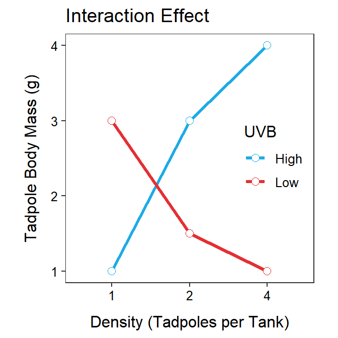
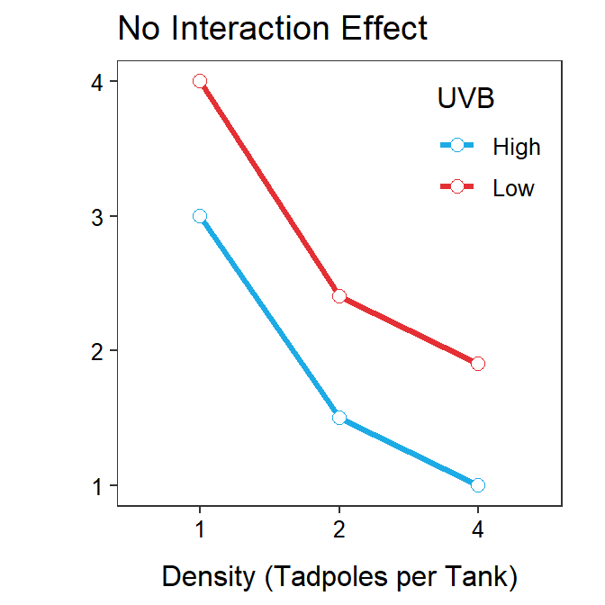
Figure 10.1: Interaction plot (mean growth rate for each treatment connected within the UV-B light intensity levels) for the tadpole experiment illustrating a hypothetical interaction effect (Left) and a lack of an interaction effect (Right).
Interaction effect: When the effect of one explanatory variable (or factor) on the mean response is significantly different among the levels of the other explanatory variable (or factor).
The tell-tale sign of an interaction effect is if you describe the effect of a factor on the mean response differently depending on the level of the other explanatory variable. For example, in Figure 10.2-Left the effect of tadpole density on mean body mass is increasing in the high UV-B light intensity treatments, but is neither increasing nor decreasing in the low UV-B light intensity treatments. The fact that density had a different effect on mean body mass in the different UV-B light treatments tells of an interaction effect. In Figure 10.2-Right mean body mass increases with increasing density but at a very different rate (at least for densities of 1 to 2 tadpoles per tank). Again, this is a different conclusion about the effect of density on mean body mass depending on level of UV-B light; thus this represents an interaction effect.
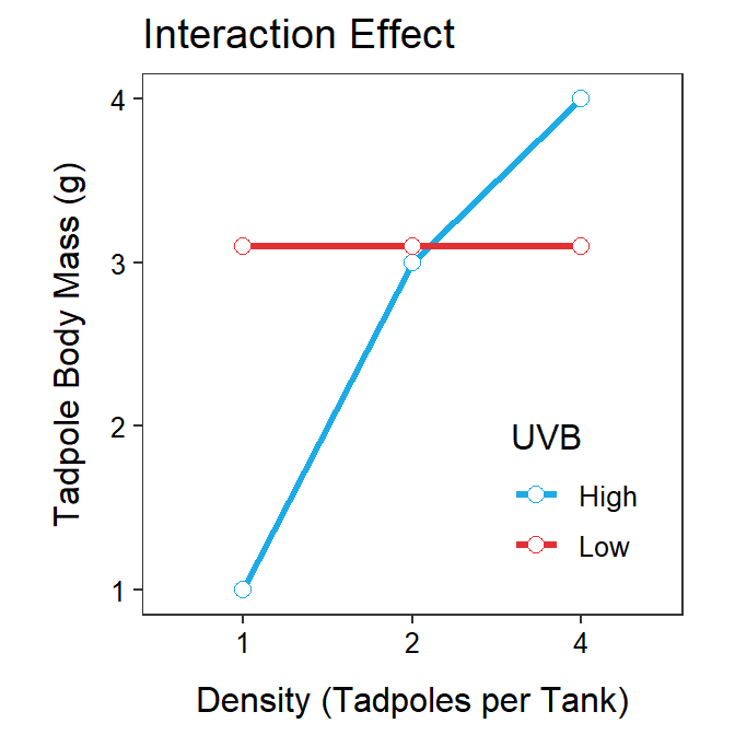
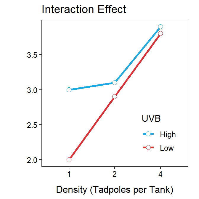
Figure 10.2: Interaction plot (mean growth rate for each treatment connected within the UV-B light intensity levels) for the tadpole experiment illustrating hypothetical interaction effects.
In Module 11 we will develop objective mathematical measures of whether an interaction effect exists.48 However, in addition to the concept above, an interaction effect will look like means that are connected for levels of one explanatory variable that “do not track together” for levels of the other explanatory variable. For example, in Figure 10.2-Left the “blue line” (connecting high UV-B light treatments) is steadily increasing whereas the “red line” (connecting low UV-B light treatments) is steadily flat – i.e., they don’t “track” together, which indicates an interaction effect. The two lines also do not track together in Figure 10.2 - Right.
An interaction effect is evident if the “lines” in an interaction plot do not largely “track together.”
10.3 Main Effects
A main effect occurs when there is a difference in the mean response among levels of an explanatory variable that is consistent across the levels of the other explanatory variable. Thus, by definition, a main effect cannot exist if an interaction effect exists. Thus, do not try to identify main effects when an interaction effect is present.
Do not identify main effects when an interact effect exists.
For example, Figure 10.1-Right showed no significant interaction; thus, main effects can be assessed. In that case, the main effect of density is that mean body mass decreased when density increased from 1 to 2 tadpoles per tank and continued to decrease at a slower rate when the density increased from 2 to 4 tadpoles per tank. From the same figure, the effect of UV-B light density is that mean body mass was greater at a low than at a high UV-B intensity.49
Main effects can also be determined for both interaction plots in Figure 10.3. The main effect for density in Figure 10.3-Left is the same as that described for Figure 10.1-Right. However, in this case there is no UV-B main effect because there is no separation in means by UV-B light level at each level of density. In other words the red line for low UV-B light and the blue line for high UV-B light are (nearly) directly on top of each other, so there is no difference in means due to UV-B light and thus no main effect of UV-B light.
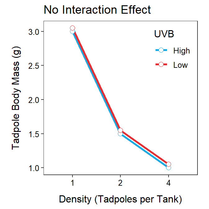
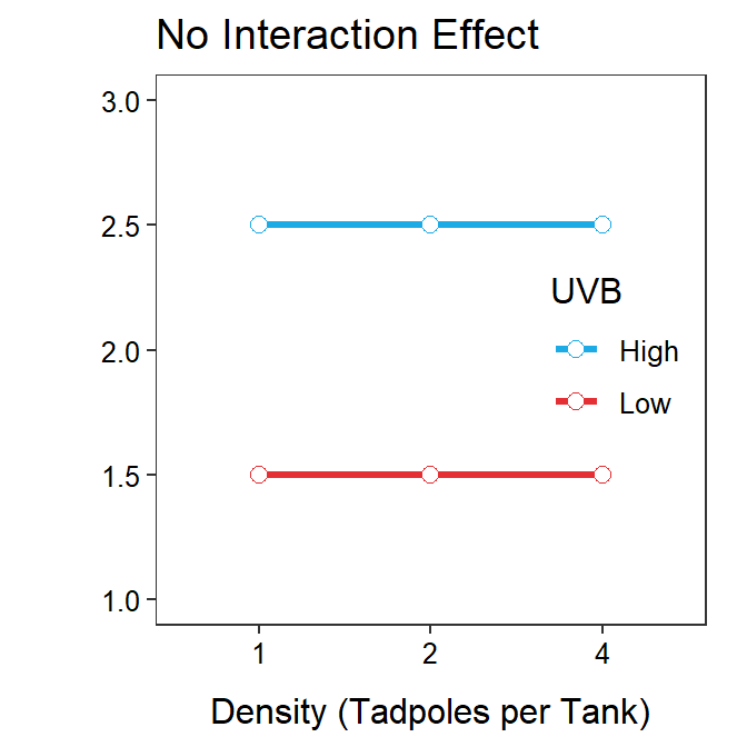
Figure 10.3: Interaction plot (mean growth rate for each treatment connected within the UV-B light intensity levels) for the tadpole experiment illustrating hypothetical lacks of interaction effects.
In Figure 10.3-Right, there is no main effect of tadpole density as the mean body mass at each density within each UV-B light level is the same; i.e., mean body mass does not differ by density. However, there is a UV-B light main effect as mean body mass at the high UV-B light intensity is always50 greater than mean body mass at the low UV-B light intensity.
As a reminder, only assess main effects if there is no interaction effect. Visually a main effect of the factor shown on the x-axis will be evident if the lines connecting the means are not horizontal (i.e., the means differ). In contrast, a main effect of the factor not shown on the x-axis (but shown as a legend) will be evident if the lines connecting the means are not right on top of each other.
10.4 Advantages of CCFD
A two-factor CCFD has two major advantages over two separate OFAT experiments.
First, the CCFD allocates individuals more efficiently than the two OFAT experiments. For example, in the CCFD of the tadpole experiment, all 90 individuals were used to identify differences among the light intensities AND all 90 individuals were used to identify differences among the densities of tadpoles. However, in the OFAT experiments, only 44 individuals51 were used to identify differences among the light intensities and only 45 individuals were used to identify differences among the tadpole densities.
Efficiency in allocation of individuals effectively leads to an increased sample size for determining the effect of any one factor. An increased sample size means more precise estimates of means52 and more statistical power. Statistical power is the probability of correctly rejecting a false null hypothesis. In lay terms, statistical power is the ability to correctly identify a difference in means when a difference in means really exists. Relatedly, the increased sample size means that smaller effect sizes can be identified. In practice this means that smaller differences in means will be found to be statistically different. In yet other words, a smaller “signal” can be detected. Finally, the increased efficiency means that the same power and detectable effect size can be obtained with a smaller overall sample size and, thus, lower costs.
A second advantage of CCFD studies is that they allow researchers to identify if an interaction effect exists between the two explanatory variables. An interaction effect cannot be detected in OFAT studies because the two explanatory variables are not considered simultaneously.
CCFD studies effectively increase the sample size for identifying effects on the response variable. More efficient use of individuals in CCFD studies results in increased power and increased ability to detect small effect sizes, or lower costs to obtain the same power and effect size detectability.
CCFD studies allow for the possible detection of an interaction effect.
The combination of levels is often called a “treatment” in an experiment. In an observational study it would just be called a “group.”↩︎
That is, we will use a p-value.↩︎
The blue line was always below the red line by roughly the same amount.↩︎
For each density.↩︎
One individual was not used in order to have equal numbers of individuals in each treatment.↩︎
That is, a reduced SE↩︎