Module 5 One-Way Foundations
Many studies, including the following examples, compare means from more than two independent populations.
- Test for differences in the mean total richness of macroinvertebrates between three zones of a river (Grubbs and Taylor 2004).
- Test if mean social capital differs among children from Estonia, Germany, and Russia (Beilmann et al. (2014)).
- Determine if the mean frequency of occurrence of badgers (Meles meles) in plots differs among plots from different locations (Virgos and Casanovas 1999).
- Determine if the mean job satisfaction rating differs among managers, superintendents, and supervisors (Magharbi 1999).
- Determine if the mean age of harvested deer (Odocoelius virginianus) differs among Ashland, Bayfield, Douglas, and Iron counties.
- Determine if mean trust in weather forecasts differs among five different types of forecasting models (Joslyn and LeClerc 2012).
In each of these situations, the mean of a quantitative variable (e.g., total richness, social capital, frequency of occurrence, job satisfaction rating, age, or trust rating) is compared among three or more populations of a single factor variable (e.g., zones, countries, locations, jobs, counties, or forecasting models). A 2-sample t-test cannot be used in these situations because more than two groups are compared. A one-way analysis of variance (or one-way ANOVA) is an extension of a 2-sample t-test that can be used for each of these situations.19
A one-way analysis of variance (ANOVA) is used to determine if a significant difference exists among the means of two or more populations.
In this module, we examine the immunoglobulin20 measurements of opossums (imm) during three months of the same year (season). The data are loaded into R and a subset of rows is shown below.
opp <- read.csv("Opossums.csv")headtail(opp)#R> imm season
#R> 1 0.640 feb
#R> 2 0.680 feb
#R> 3 0.731 feb
#R> 25 0.490 nov
#R> 26 0.333 nov
#R> 27 0.492 novData must be stacked!!
5.1 Analytical Foundation
The generic null hypothesis for a one-way ANOVA is
\[ \text{H}_{\text{0}}: \mu_{1} = \mu_{2} = \ldots = \mu_{I} \]
where \(I\) is the total number of groups or populations.21 The alternative hypothesis for a one-way ANOVA is “wordy” and is often written as
\[ \text{H}_{\text{A}}:``\text{At least one pair of means is different''} \]
because not all pairs of means need differ for the null hypothesis to be rejected. Thus, rejecting H0 in favor of HA is a statement that some difference in group means exists. It does not indicate which group means differ.22
Rejecting H0 means that some group means differ.
The simple (\(Y_{ij} = \mu + \epsilon_{ij}\)) and full (\(Y_{ij} = \mu_{i} + \epsilon_{ij}\)) models for the one-way ANOVA are the same as those for the 2-sample t-test, except that \(I\) may be >2 means in the full model. Thus, SSTotal, SSWithin, and SSAmong; dfTotal (=\(n\)-1), dfWithin (=\(n\)-\(I\)). and dfAmong (=\(I\)-1); and MS, F, and p-values are all computed using the same formulae shown in Module 4, except to again note that \(I\)≥2.23
A 2-Sample t-Test is simply a special case of a One-Way ANOVA.
Figure 5.1 is a visual representation of the simple and full models of a One-Way ANOVA, along with residuals from each. Note the similarity with figures from the Module 4, except that there are three group means here.
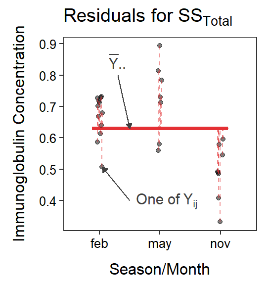
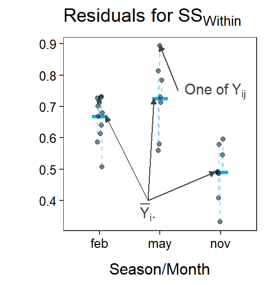
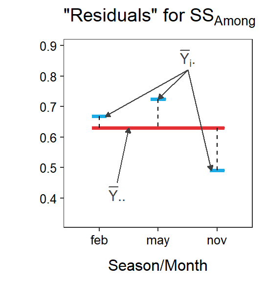
Figure 5.1: Immunoglobulin concentrations versus season (or month) of capture for New Zealand opposums. The grand mean is shown by a red horizontal segment, group means are shown by blue horizontal segments, residuals from the grand mean are red vertical dashed lines, residuals from the groups means are blue vertical dashed lines, and differences between the group means and the grand mean are black vertical dashed lines.
An ANOVA table (Table 5.1) is used to display the results from a one-way ANOVA.
| Df | Sum Sq | Mean Sq | F value | Pr(>F) | |
|---|---|---|---|---|---|
| season | 2 | 0.2340 | 0.1170 | 14.4486 | 1e-04 |
| Residuals | 24 | 0.1944 | 0.0081 |
In addition to the usual meanings attached to MSAmong, MSWithin, and MSTotal,24 the following can be discerned from this ANOVA table.
- dfAmong=2 and, because dfAmong=\(I\)-1, then \(I\)=3. This confirms that there are three groups in this analysis.
- dfTotal=dfAmong+dfWithin=2+24=26. Because dfTotal=\(n\)-1, then \(n\)=27. This shows that there are 27 individuals in this analysis.
- There is a significant difference in the mean immunoglobulin values among the three months because the p-value=0.0001<α.
5.2 One-Way ANOVA in R
The models for a one-way ANOVA are fit and assessed with lm() exactly as described for a 2-sample t-test in Section 4.8.25
lm1 <- lm(imm~season,data=opp)
anova(lm1)
#R> Analysis of Variance Table
#R>
#R> Response: imm
#R> Df Sum Sq Mean Sq F value Pr(>F)
#R> season 2 0.23401 0.117005 14.449 7.609e-05
#R> Residuals 24 0.19435 0.008098A graphic that illustrates the mean immunoglobulin value with 95% confidence intervals for each month is constructed below (as shown in Section 2.2).
ggplot(data=opp,mapping=aes(x=season,y=imm)) +
  geom_jitter(alpha=0.5,width=0.05) +
  stat_summary(fun.data=mean_cl_normal,geom="errorbar",size=2,width=0) +
  stat_summary(fun=mean,geom="point",pch=21,fill="white",size=2) +
  labs(x="Season/Month",y="Immunoglobulin Concentration") +
  theme_NCStats()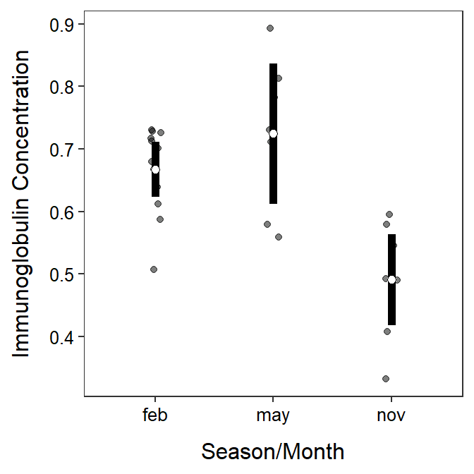
This and the next several modules depends heavily on the foundational material in Modules 1-4, especially the concepts of simple and full models; “signal” and “noise”; variances explained and unexplained; and SS, MS, F, and p-values.↩︎
Any of a class of proteins present in the serum and cells of the immune system, which function as antibodies.↩︎
From this, it is evident that the one-way ANOVA is a direct extension of the 2-sample t-test.↩︎
Methods to identify which group means differ are in Module 6.↩︎
The MS, F, and p-value are computed the same in nearly every ANOVA table encountered in this class.↩︎
Note that MSTotal must be computed from SSTotal and dfTotal and not by summing MSAmong an MSWithin.↩︎
As a reminder,
response~factoris the first argument and a data frame is given indata=inlm(), the results oflm()should be assigned to an object, and the ANOVA table is extracted withanova().↩︎