Module 21 IVR Models & Sub-Models
Covariate, indicator, and interaction variables (see Module 20) can be entered into a single model that will allow one to determine if simple linear regression lines differ among groups. As such, possible differences among slopes, intercepts, or both can be determined. In this module, the model for this Indicator Variable Regression (IVR) analysis is introduced. Hypothesis testing for slopes and intercepts is introduced in Module 22.
21.1 Ultimate Full Model
Consider the situation introduced in Module 20 where researchers examined the effect of salmon weight on mirex concentration in the tissue for two species of salmon (Coho and Chinook). In this case, there is one quantitative response variable (\(MIREX\)), one covariate (\(WEIGHT\)), and one indicator variable (\(COHO\)) generated from a factor variable with only two categories (i.e., species). In addition, there is an interaction variable between \(WEIGHT\) and \(COHO\).
The ultimate full model for this situation is
\[ \mu_{MIREX|WEIGHT,COHO} = \alpha+\beta WEIGHT+\delta_{1}COHO+\gamma_{1}WEIGHT:COHO \]
where \(\mu_{MIREX|WEIGHT,COHO}\) is read as “mean MIREX at a given values of the WEIGHT and COHO variables.” This is called the ultimate full model because the model cannot get more complicated for this situation as all variables of interest are included in the model. In subsequent modules, simpler models with fewer variables (and parameters) will also be considered.
Specific parameters are used in the ultimate full model of an IVR as shown above. Specifically, they are
- \(\alpha\): an overall intercept term.
- \(\beta\): coefficient on the covariate.
- \(\delta_{i}\): coefficient on the \(i\)th indicator variable.
- \(\gamma_{i}\): coefficient on the interaction between the covariate and the \(i\)th indicator variable.
Each of these parameters has a specific meaning or interpretation that will be better understood by reducing the ultimate full model to its constituent sub-models.
The covariate, indicator, and interaction variables are entered in that order into the ultimate full model of an IVR to allow for consistent and simple interpretations.
21.2 Sub-Models
The ultimate full model in IVR contains sub-models that are SLR models for each group represented by the indicator variables. The sub-models can be revealed by substituting appropriate values for the indicator variables in the ultimate full model. For example \(COHO=0\) for the “non-Coho” group (i.e., Chinook). Thus, to find the sub-model for Chinook Salmon, plug 0 for \(COHO\) in the ultimate full model and simplify.
\[ \begin{split} \mu_{MIREX|WEIGHT,COHO} &= \alpha+\beta WEIGHT+\delta_{1}COHO+\gamma_{1}WEIGHT:COHO \\ \vdots\;\;\;\;\;\;\;\;\;\;\;\;\;\;\;\;&=\alpha+\beta WEIGHT+\delta_{1}0+\gamma_{1}WEIGHT:0\\ \vdots\;\;\;\;\;\;\;\;\;\;\;\;\;\;\;\;&=\alpha+\beta WEIGHT+0+0\\ \mu_{MIREX|WEIGHT,COHO}&=\alpha+\beta WEIGHT\\ \end{split} \]
Similarly, the sub-model for Coho is found by plugging 1 for \(COHO\) in the ultimate full model and simplifying.
\[ \begin{split} \mu_{MIREX|WEIGHT,COHO} &= \alpha+\beta WEIGHT+\delta_{1}COHO+\gamma_{1}WEIGHT:COHO \\ \vdots\;\;\;\;\;\;\;\;\;\;\;\;\;\;\;\;&=\alpha+\beta WEIGHT+\delta_{1}1+\gamma_{1}1WEIGHT \\ \vdots\;\;\;\;\;\;\;\;\;\;\;\;\;\;\;\;&=\alpha+\beta WEIGHT+\delta_{1}+\gamma_{1}WEIGHT \\ \vdots\;\;\;\;\;\;\;\;\;\;\;\;\;\;\;\;&=\alpha+\delta_{1}+\beta WEIGHT+\gamma_{1}WEIGHT \\ \mu_{MIREX|WEIGHT,COHO} &=(\alpha+\delta_{1})+(\beta+\gamma_{1})WEIGHT \\ \end{split} \]
These sub-models are appended to the tables from Module 20 to provide a succinct summary.
| Species | COHO | Sub-Model (\(\mu_{MIREX|WEIGHT}=\)) |
|---|---|---|
| Chinook (Reference) | 0 | \(\alpha+\beta WEIGHT\) |
| Coho | 1 | \((\alpha+\delta_{1})+(\beta+\gamma_{1})WEIGHT\) |
Examination of the sub-models for each group shows that each sub-model is itself an SLR model. The sub-model for Chinook Salmon is an SLR with a slope of \(\beta\) and intercept of \(\alpha\). In contrast, the sub-model for Coho Salmon is an SLR with a slope of \(\beta+\gamma_{1}\) and intercept of \(\alpha+\delta_{1}\).
The process is similar when there are more than two groups, except that 0s and 1s must be substituted for multiple indicator variables. For example, the ultimate full model for the situation when three years (1977, 1982, 1986) were considered is
\[ \begin{split} \mu_{MIREX|WEIGHT,\cdots} = & \; \alpha+\beta WEIGHT + \delta_{1}YEAR1982 + \delta_{2}YEAR1986 + \\ & \; \gamma_{1}WEIGHT:YEAR1982 + \gamma_{2}WEIGHT:YEAR1986 \\ \end{split} \]
To find the sub-model for 1982, for example, requires plugging 1 in for \(YEAR1982\) and 0 for \(YEAR1986\) and simplifying.93
\[ \begin{split} \mu_{MIREX|WEIGHT,\cdots} &= \alpha+\beta WEIGHT + \delta_{1}1 + \delta_{2}0 + \gamma_{1}WEIGHT:1 + \gamma_{2}WEIGHT:0 \\ \vdots\;\;\;\;\;\;\;\;\;\;\;\;\;\;\;\;&= \alpha+\beta WEIGHT + \delta_{1} + 0 + \gamma_{1}WEIGHT + 0 \\ \mu_{MIREX|WEIGHT,\cdots}&= (\alpha+\delta_{1}) + (\beta+\gamma_{1})WEIGHT \end{split} \]
A similar process can be used to find the sub-models for 1977 and 1986.94 The sub-models are then summarized in the following table.
| Year | YEAR1982 | YEAR1986 | Sub-Model (\(\mu_{MIREX|WEIGHT}=\)) |
|---|---|---|---|
| 1977 (Reference) | 0 | 0 | \(\alpha+\beta WEIGHT\) |
| 1982 | 1 | 0 | \((\alpha+\delta_{1})+(\beta+\gamma_{1})WEIGHT\) |
| 1986 | 0 | 1 | \((\alpha+\delta_{2})+(\beta+\gamma_{2})WEIGHT\) |
Once again, each sub-model is itself an SLR model. For example, the slopes are \(\beta\), \(\beta+\gamma_{1}\), and \(\beta+\gamma_{2}\) for the years 1977, 1982, and 1986, respectively.
Sub-models are found by appropriately substituting “0”s and “1”s for the indicator variable(s) in the IVR ultimate full model and simplifying.
Each sub-model is an SLR for one of the groups represented in the IVR ultimate full model.
The sub-model for the reference group is always \(\mu_{Y|X}=\alpha+\beta X\). The slopes for the other groups always have a \(\gamma_{i}\) added to \(\beta\) and the intercepts always have a \(\delta_{i}\) added to \(\alpha\).
21.3 Interpreting Parameter Estimates
Careful examination of the sub-models in the tables above help illustrate what the model parameters (i.e., \(\alpha\), \(\beta\), \(\delta_{i}\), and \(\gamma_{i}\)) mean. The sub-model for the reference groups is always \(\mu_{Y|X}=\alpha+\beta X\); thus, \(\alpha\) is the intercept and \(\beta\) is the slope for the reference group. From above, it is also evident that the intercept for the \(i\)th group is \(\alpha+\delta_{i}\) and the slope for the \(i\)th group is \(\beta+\gamma_{i}\).
To understand \(\delta_{i}\), consider the following algebra for the difference in intercepts between the \(i\)th group and the reference group.
\[ i\text{th Group's Intercept} - \text{Reference Group's Intercept} = (\alpha+\delta_{i}) - \alpha = \delta_{i} \]
Thus, \(\delta_{i}\) is the additive difference between intercepts for the \(i\)th and reference groups. Similar algebra shows that \(\gamma_{i}\) is the additive difference in slopes between the \(i\)th group and the reference group.
\[ i\text{th Group's Slope} - \text{Reference Group's Slope} = (\beta+\gamma_{i}) - \beta = \gamma_{i} \]
In summary, the parameters in the ultimate full model have the following interpretations (see Figure 21.1).
- \(\alpha\): y-intercept for the reference group.
- \(\beta\): slope for the reference group.
- \(\delta_{i}\): difference in y-intercepts between the \(i\)th group and the reference group.
- \(\gamma_{i}\): difference in slopes between the \(i\)th group and the reference group.
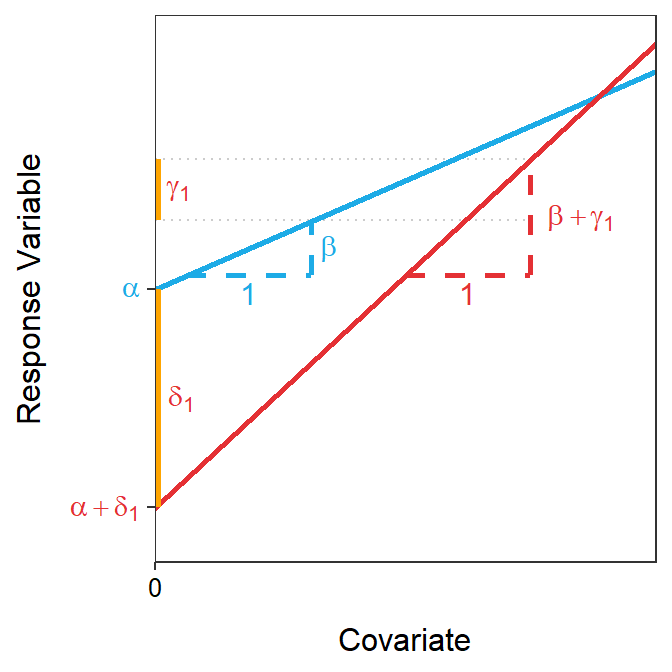
Figure 21.1: Representation of two sub-models fit with the ultimate full model in an IVR with the geometric meaning of each parameter. The blue line is the sub-model for the reference group. Note that \(\alpha\)=2, \(\beta\)=0.4, \(\delta_{1}\)=-1.6, and \(\gamma_{1}\)=0.45 in this example.
These interpretations show why the first group is called the reference group. The parameters in the reference sub-model represent the intercept and slope for that group. These parameters also appear in the other sub-models, but each has another parameter added to it to account for differences between the non-reference group and the reference group. In other words, every difference in slopes or intercepts is computed relative to the slope or intercept for the reference group. Thus, \(\delta_{i}\) and \(\gamma_{i}\) are only meaningful relative to the reference group.
Coefficients on indicator variables (i.e., the \(\delta_{i}\)) always measure differences in intercepts between a non-reference group and the reference group.
Coefficients on interaction variables (i.e., the \(\gamma_{i}\)) always measure differences in slopes between a non-reference group and the reference group.
The ultimate full model of an IVR can represent four situations between two groups depending on values of the \(\delta_{i}\) and \(\gamma_{i}\) parameters. These four situations are depicted in Figure 21.2 for just two groups.
- Completely Separate Lines: Two completely separate lines are needed for both groups (i.e., \(\delta_{1}\neq0\) and \(\gamma_{1}\neq0\)).
- Same Intercept: Separate non-parallel lines with the same y-intercept are needed for both groups (i.e., \(\delta_{1}=0\) and \(\gamma_{1}\neq0\))
- Parallel Lines: Separate parallel lines with different y-intercepts are needed for both groups (i.e., \(\delta_{1}\neq0\) and \(\gamma_{1}=0\)).
- Coincident Lines: A single regression line represents the relationship between the response variable and the covariate for both groups (i.e., \(\delta_{1}=0\) and \(\gamma_{1}=0\)).
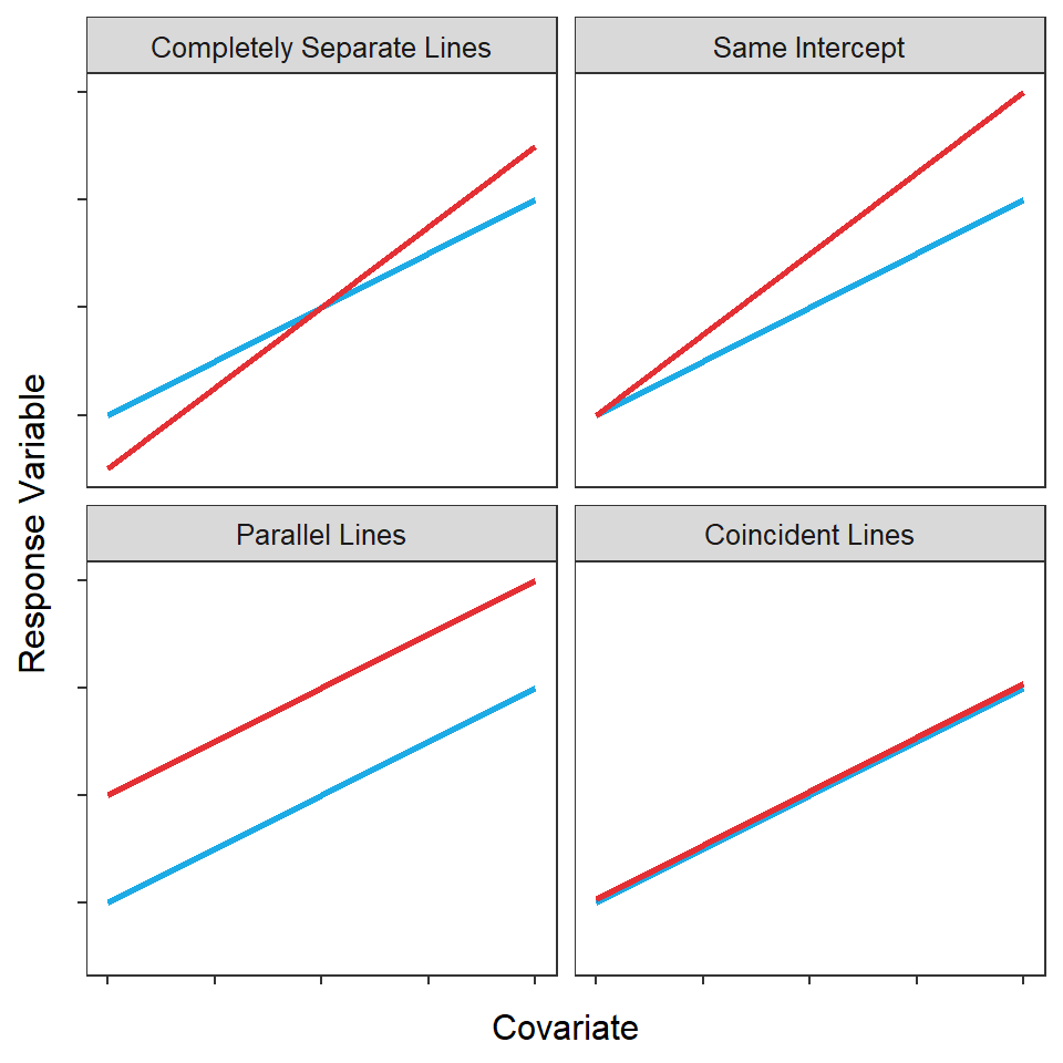
Figure 21.2: Hypothetical depictions of four situations that can occur for the relationship between a response variable and a covariate for two groups.
21.4 Ultimate Full Model in R
Fitting the ultimate full model in R is straightforward because it is essentially the same as fitting a Two-Way ANOVA (see 12.1) and R automatically creates the indicator variables behind the scenes. The ultimate full model for an IVR is fit in lm() with response~covariate+factor+covariate:factor,95 with the variables on the right-hand-side in that order to match what was done above.
ivr1 <- lm(mirex~weight+species+weight:species,data=Mirex)Extracting Parameter Estimates
The parameter estimates and their confidence intervals are extracted with coef() and confint() as before.
cbind(Ests=coef(ivr1),confint(ivr1))#R> Ests 2.5 % 97.5 %
#R> (Intercept) 0.135 0.093 0.178
#R> weight 0.010 0.004 0.015
#R> speciescoho -0.051 -0.113 0.011
#R> weight:speciescoho 0.012 -0.001 0.025Parameter estimates under the “Ests” column are in rows that are generally labeled as the variables in the ultimate full model. Note that R prepends the indicator variable with the name of the original factor variable; i.e., speciescoho instead of COHO. From this then, \(\hat{\alpha}\)=0.135, \(\hat{\beta}\)=0.010, \(\hat{\delta}_{1}\)=-0.051, and \(\hat{\gamma}_{1}\)=0.012. Thus, for example, the sample slope for Chinook Salmon (the reference groups) is 0.010 and the sample slope for Coho Salmon is 0.012 greater than the sample slope for Chinook Salmon. Furthermore, for example, one is 95% confident that \(\beta\) is between 0.004 and 0.015 and \(\gamma_{1}\) is between -0.001 and 0.025.
Of course, inferential methods are needed to determine if these results suggest a real difference in parameters between populations. For example, a statistical test of whether \(\gamma_{1}=0\) would be used to determine if the population slopes differed between Coho and Chinook salmon. These types of tests are introduced in Module 22.
Fitted Line Plots
A visual of the fitted IVR model is constructed the same as the visual for an SLR model except that the color of the points and the regression line for each group is mapped to the factor variable. The plotting character and colors should then be removed from geom_point(). For example, note the color=species in mapping=aes() and the simplicity of geom_point() in the code below.
ggplot(data=Mirex,mapping=aes(x=weight,y=mirex,color=species)) +
  geom_point() +
  labs(x="Weight (kg)",y="Mirex Concentration (mg/kg)") +
  theme_NCStats() +
  geom_smooth(method="lm",se=FALSE)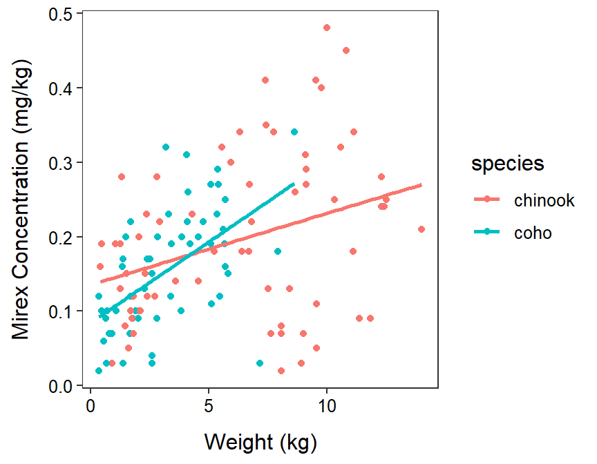
From this plot, note that the intercept for Coho is less than the intercept for Chinook (as you would expect because \(\hat{\delta}_{1}\)=-0.051) and the slope for Coho is greater than (i.e., steeper) than that for Chinook (as you would expect because \(\hat{\gamma}_{1}\)=0.012)
Predictions
Predicted values for IVR models are constructed by submitting the lm() object and a data frame of observed values of the explanatory variables to predict(), as was described for SLR models (see Section 15.7). One must make sure, though, that the data frame contains an observed value for each explanatory variable found in the lm() object.
For example, the predicted value, with a 95% prediction interval, for a 3 kg Coho Salmon is found with
nd <- data.frame(weight=3,species="coho")
predict(ivr1,newdata=nd,interval="prediction")
#R> fit lwr upr
#R> 1 0.1496893 -0.03240232 0.331781Similarly, the predicted values, with 95% prediction intervals, for a 5 kg Chinook AND a 3 kg Coho Salmon are found with
nd <- data.frame(weight=c(5,3),species=c("chinook","coho"))
predict(ivr1,newdata=nd,interval="prediction")
#R> fit lwr upr
#R> 1 0.1834880 0.001557795 0.3654182
#R> 2 0.1496893 -0.032402319 0.3317810The results may be easier to read if you bind together the new data.frame and the prediction results.
nd <- data.frame(weight=c(5,3),species=c("chinook","coho"))
cbind(nd,predict(ivr1,newdata=nd,interval="prediction"))
#R> weight species fit lwr upr
#R> 1 5 chinook 0.1834880 0.001557795 0.3654182
#R> 2 3 coho 0.1496893 -0.032402319 0.3317810