Module 25 Foundational Principles
Logistic regression models are used when a researcher is investigating the relationship between a binary categorical response variable and a quantitative explanatory variable.106 Typically, logistic regression is used to predict the probability of membership in one level of the response variable given a particular value of the explanatory variable. Binary107 logistic regression would be used in each of the following situations:
- Predict the probability that a bat is of a certain subspecies based on the size of the canine tooth.
- Predict the probability that a household will accept an offer to install state-subsidized solar panels given the household’s income.
- Predict the probability that a beetle will die when exposed to a certain concentration of a chemical pollutant.
- Predict the probability of mortality for a patient given a certain “score” on a medical exam.
Binary Logistic Regression: A linear model where a binary response variable (i.e., two possible outcomes) is examined with a quantitative explanatory variable.
25.1 Need for a Transformation
The response variable in a logistic regression is categorical. How do you make a plot with categorical data on the y-axis? How do you construct a “regression” model when the y-axis variable is categorical?
In this course, we will only consider binary response variables; i.e., only two categories. The two categories will generically be labeled as “success” and “failure,” where success and failure is defined by the researcher. For example, a researcher may be interested in the probability of a heart attack and, thus, would define a “success” as having a heart attack.
The binary response variable in a logistic regression will be treated as an indicator variable, where a “success” is coded as a “1” and a “failure” is coded as a “0.”108 Treating this variable as “quantitative” will allow us to use techniques from previous modules.
However, fitting a linear regression to this response variable plotted against the quantitative explanatory variable immediately exposes two problems (Figure 25.1). First, the linearity (and homoscedasticity) assumptions of linear regression are not met. Second, predicted probabilities from this model can be less than 0 and greater than 1, even within the observed domain of the explanatory variable. Clearly, a linear regression cannot be used to model this type of data.
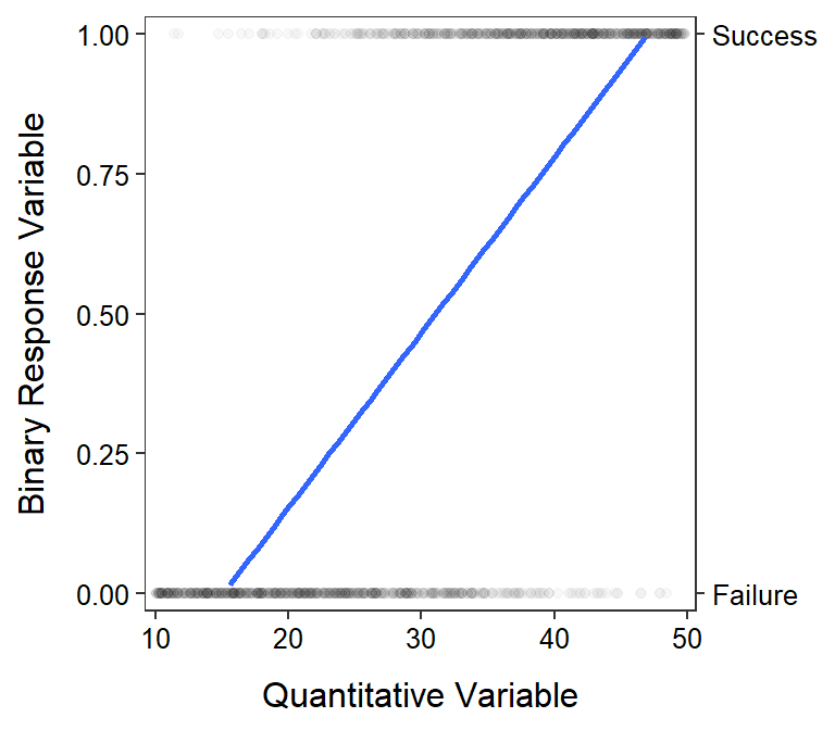
Figure 25.1: Plot of the binary response variable, as an indicator variable, versus a quantitative explanatory variable with the best-fit linear regression line super-imposed. Note that darker points have more individuals over-plotted at that coordinate.
Recall that all previous linear models dealt with the mean of the response variable. Logistic regression is no different in that it attempts to model the mean of \(Y\) at each value of \(X\). As a simple example consider the five observations of “success” and “failure” below at one particular value of \(X\), where \(Z\) is the indicator variable that corresponds to \(Y\).
 X    Y      Z
20  Success  1
20  Failure  0
20  Failure  0
20  Success  1
20  Success  1
In this example the mean of \(Z\) is \(\frac{1+0+0+1+1}{5}\)=\(\frac{3}{5}\)=0.6. Lets also calculate the proportion of “successes” in \(Y\) as \(\frac{\text{Number of Successes}}{\text{Total Number of Observations}}\)=\(\frac{3}{5}\)=0.6. Thus, because \(0\)s and \(1\)s are used in the indicator variable, the mean of the indicator variable is the same as the probability of success for the corresponding factor variable.
In many situations it is hard to visualize the probability of success versus the explanatory variable because few values of \(X\) have multiple observations of \(Y\). Thus, a visual is constructed by computing the probability of success (\(p_{i}\)) within \(i\) “windows” of \(X\) values. For example, Figure 25.2 shows the probability of success calculated within “windows” of \(X\) that are 2.5 units wide.
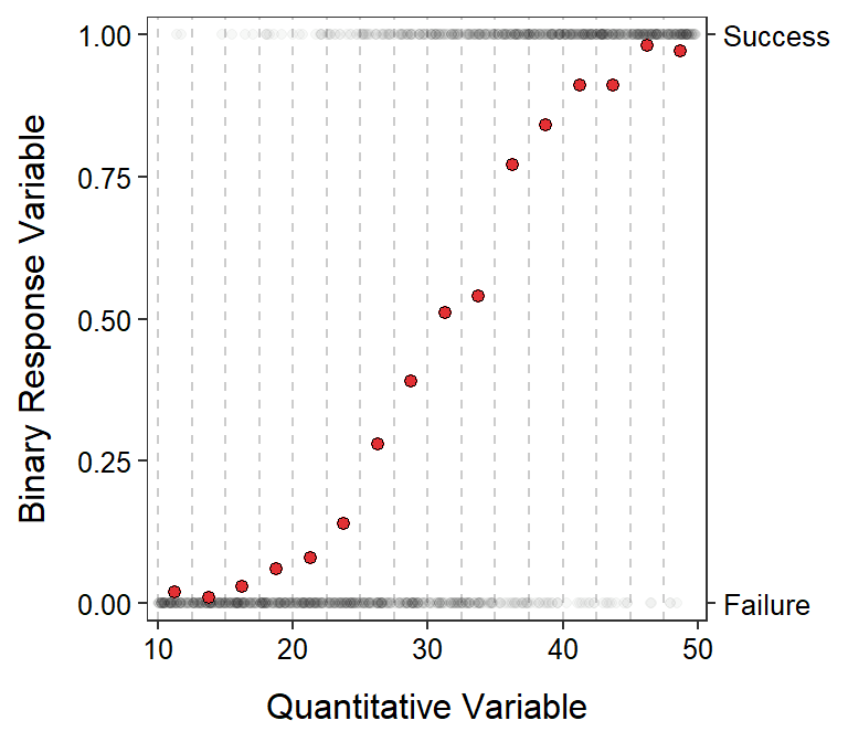
Figure 25.2: Plot of the binary response variable, as an indicator variable, versus a quantitative explanatory variable with the vertical lines representing ‘windows’ in which the probability of ‘success’ (red circles) were calculated. These are the same data as in the previous figure.
From Figure 25.2, it is obvious that a model for the probability of “success” is non-linear. As is usual, when the assumptions of a model are not met then a transformation is considered. The transformation required for a logistic regression is introduced in the next two sections.
In logistic regression the probability of success is modeled, which is the same as modeling the mean of \(Y\) at given values of \(X\).
25.2 Odds
The first step in transforming probabilities of success is to calculate odds of success. The odds of “success” is the probability of “success” divided by the probability of “failure”; i.e.,
\[ odds_{i} = \frac{p_{i}}{1-p_{i}} \]
For example, an odds of 5 means that the probability of “success” is five times more likely than the probability of “failure.” In contrast, an odds of 0.2 means that the probability of “failure” is five times (i.e., \(\frac{1}{0.2}\)=5) more likely than the probability of “success.”
Odds: The ratio of the probability of “success” to the probability of “failure.”
Odds have two important characteristics. First, an odds of 1 means that the probability of “success” is the same as the probability of “failure.” Second, odds are bounded below by 0 (i.e., negative odds are impossible) but are not bounded above (i.e., odds can increase to positive infinity; Figure 25.3).
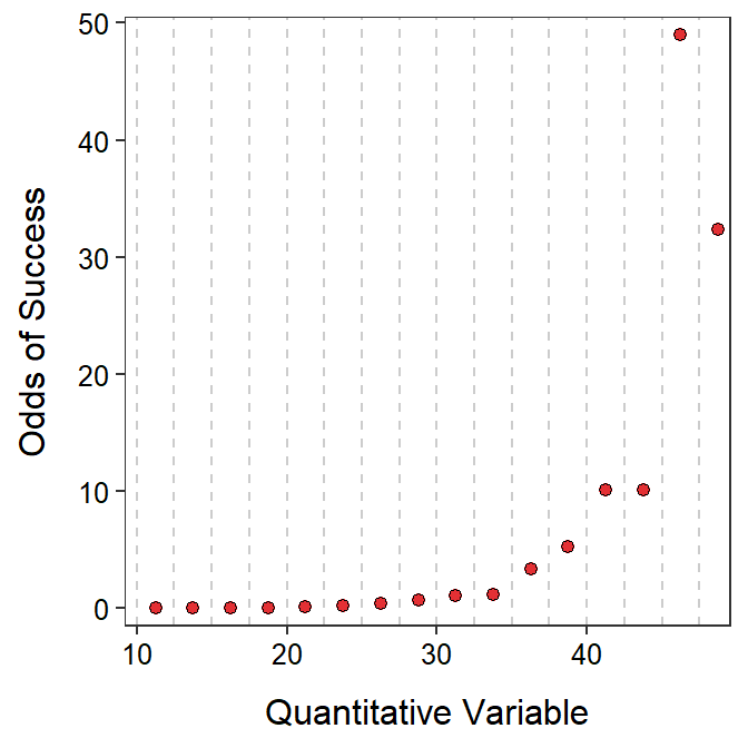
Figure 25.3: Plot of the odds of ‘success’ for the same probabilities of ‘success’ in the previous figure.
Plotting odds versus the explanatory variable is still not linear (Figure 25.3). Thus, odds still need to be transformed before a linear model can be fit.
25.3 Log Odds and the Logit Transformation
While the plot of the odds of “success” versus the quantitative explanatory variable is not linear, it does have the characteristic shape of an exponential function (Figure 25.3). Exponential functions are “linearized” by log transforming the response variable (see Section 18.1.2). The log of the odds is called the “logit” transformation of the probability of “success.” Thus,
\[ logit(p_{i}) = log(odds_{i}) = log\left(\frac{p_{i}}{1-p_{i}}\right) \]
The plot of \(logit(p_{i})\) versus the explanatory variable is generally linear (Figure 25.4).
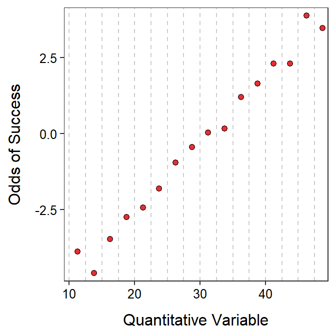
Figure 25.4: Plot of the log odds of ‘success’ (i.e., the logit transformed probability of ‘success’) for the same odds of ‘success’ in the previous figure.
Therefore, the logit transformation is a common transformation for “linearizing” the relationship between the probability of “success” and the quantitative explanatory variable. The logit transformation is the basis for a logistic regression, such that the logistic regression model is
\[ log\left(\frac{p_{i}}{1-p_{i}}\right) = \alpha + \beta x_{i} \]
where \(\alpha\) is the “intercept” parameter and \(\beta\) is the “slope” parameter.
25.4 Back-Transformation Introduction
While it will be discussed more in the next modules, it is evident from the logistic regression model above that that model is used to predict log odds. However, log odds are largely uninterpretable and should be back-transformed to the odds by exponentiating (i.e., \(\text{odds}=e^{\text{log(odds)}}\)).
An equation for predicting the probability of success can also be obtained with algebra, starting with the logistic regression equation.
\[ \begin{split} log\left(\frac{p}{1-p}\right) &= \alpha+\beta X \\ \frac{p}{1-p} &= e^{\alpha+\beta X} \\ p &= (1-p)e^{\alpha+\beta X} \\ p &= e^{\alpha+\beta X}-pe^{\alpha+\beta X} \\ p + pe^{\alpha+\beta X} &= e^{\alpha+\beta X} \\ p\left(1+e^{\alpha+\beta X}\right) &= e^{\alpha+\beta X} \\ p &= \frac{e^{\alpha+\beta X}}{1+e^{\alpha+\beta X}} \\ \vdots \; &= \frac{e^{log(odds)}}{1+e^{log(odds)}} \\ p &= \frac{\text{odds}}{1+\text{odds}} \end{split} \]
Thus, a probability can be calculated from the odds with \(p=\frac{\text{odds}}{1+\text{odds}}\). These relationships will be expanded upon in the next module.
Strictly, a logistic regression can be used with a categorical explanatory variable or multiple explanatory variables of mixed types. We will focus on the simplest situation where there is only one quantitative explanatory variable.↩︎
This qualifying statement is needed as not all logistic regressions have a response variable with only two levels.↩︎
See Section 20.1 for more discussion about indicator variables.↩︎