Module 14 SLR Foundational Principles
Simple linear regression (SLR) is used when a single quantitative response and a single quantitative explanatory variable are considered. The goals of SLR are to use the explanatory variable to (1) predict future values of the response variable and (2) explain the variability of the response variable. A simple linear regression would be used in the following situations.
- Evaluate the variability of porcupine body mass based on days since the beginning of winter.
- Predict daily energy consumption from the body weight of penguins.
- Explain the variability in product sales from the price of the product.
- Explain variability in a measure of “interpersonal avoidance” and a reported self-esteem metric.
- Explain variability in number of deaths related to lung cancer and per capita cigarette sales.
- Predict change in duck abundance from the loss of wetlands.
- Explain variability in a pitcher’s earned run “average” (ERA) and the average pitch speed at the point of release.
- Evaluate the variability in clutch size relative to length of female spiders.
The Data
Throughout the SLR modules, an example data set will be used that is the actual mean air temperatures and altitude lapse rates taken during the winter at eleven locations at various altitudes on Mount Everest. The “altitude lapse rate” is an index that was designed to be related to air temperature but adjusted for altitude. In this case, the researchers are testing to see if this index can be used to adequately predict the actual air temperature. Thus, actual air temperature is the response variable and altitude lapse rate is the explanatory variable.
| Altitude | MeanAirTemp | Season |
|---|---|---|
| 2076 | 10.36 | Winter |
| 2552 | 9.64 | Winter |
| 2578 | 6.07 | Winter |
| 2632 | 5.14 | Winter |
| 2857 | 6.57 | Winter |
| 2865 | 3.71 | Winter |
| 3009 | 3.14 | Winter |
| 3574 | 1.36 | Winter |
| 3978 | -0.07 | Winter |
| 4220 | -3.79 | Winter |
| 5018 | -6.07 | Winter |
14.1 Equation of a Line
Both goals of SLR are accomplished by finding the model67 that best fits the relationship between the response and explanatory variables.68 When examining statistical regression models, the most common expression for the equation of the best-fit line is
\[ \mu_{Y|X} = \alpha + \beta X \]
where \(Y\) is the response variable, \(X\) is the explanatory variable, \(\alpha\) is the y-intercept, and \(\beta\) is the slope. The \(\mu_{Y|X}\) is read as “the mean of Y at a given value of X.” The \(\mu_{Y|X}\) is used because the best-fit line models the mean values of \(Y\) at each value of \(X\) rather than the individuals themselves. This model is for the population and thus, \(\alpha\) and \(\beta\) are the population y-intercept and slope, respectively.
The equation of the best-fit line determined from the sample is
\[ \hat{\mu}_{Y|X} = \hat{\alpha} + \hat{\beta}X \]
where a “hat” on a parameter means that the value is an estimate and thus a statistic. Therefore, \(\hat{\alpha}\) and \(\hat{\beta}\) are the sample y-intercept and slope.
Statistics like \(\hat{\alpha}\) and \(\hat{\beta}\) are subject to sampling variability (i.e., vary from sample to sample) and have corresponding standard errors (to be shown in Module 15).
14.2 Best-Fit Line
A line is simply a model for data and from that model we can make predictions for the response variable by plugging a value of \(x\) into the line equation. For example, a prediction using the \(i\)th individual’s value of \(x\) is given by \(\hat{\mu}_{Y|X=x_{i}}=\hat{\alpha}+\hat{\beta}x_{i}\), where \(\hat{\mu}_{Y|X=x_{i}}\) is read as “the predicted mean of \(Y\) when \(X\) is equal to \(x_{i}\).” Visually this prediction is found by locating the value of \(x_{i}\) on the x-axis, rising vertically until the line is met, and then moving horizontally to the y-axis. This is demonstrated in Figure 14.1 for individual #2.
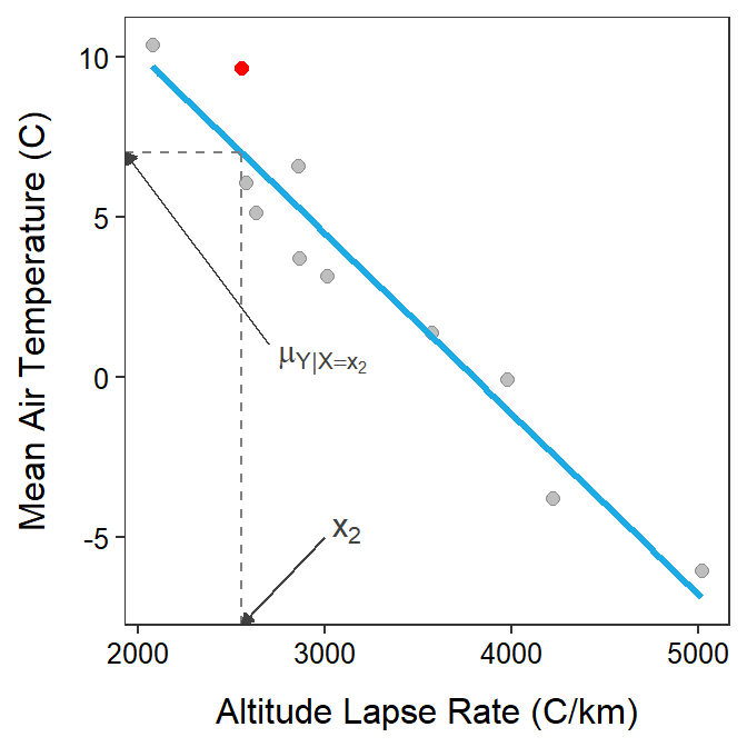
Figure 14.1: Scatterplot of actual mean air temperature versus altitude lapse rate with the best-fit line shown and the prediction demonstrated for individual 2.
As noted in previous modules, the residual is the vertical difference between an individual’s observed value of the response variable (i.e., \(y_{i}\)) and \(\hat{\mu}_{Y|X=x_{i}}\), the predicted value of the response variable using the individual’s value of the explanatory variable. Thus, a residual is \(y_{i}-\hat{\mu}_{Y|X=x_{i}}\) and measures how close the line is to that point. A residual for the second individual is demonstrated in Figure 14.2.
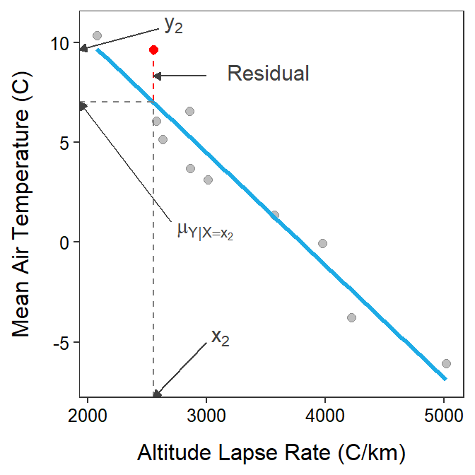
Figure 14.2: Same as previous figure except that the residual for individual #2 is highlighted with the red vertical line.
Based on previous modules, an overall measure of the lack-of-fit of the line to the data is the sum of all squared residuals; i.e.,
\[ RSS = \sum_{i=1}^{n}\left(y_{i}-\hat{\mu}_{Y|X=x_{i}}\right)^{2} \]
The best-fit line is defined by the \(\hat{\alpha}\) and \(\hat{\beta}\) out of all possible choices69 for \(\hat{\alpha}\) and \(\hat{\beta}\) that minimize the RSS (Figure 14.3).70
Figure 14.3: Scatterplot with the best-fit line (light gray) and candidate best-fit lines (blue line) and residuals (vertical red dashed lines) in the left pane and the residual sum-of-squares for all candidate lines (gray) with the current line highlighted with a red dot. Note how the candidate line is on the best-fit line when the RSS is smallest.
Mathematical statisticians have proven that the \(\hat{\beta}\) and \(\hat{\alpha}\) that minimize the RSS are given by
\[ \hat{\beta}=r\frac{s_{Y}}{s_{X}} \]
and
\[ \hat{\alpha} = \overline{Y}-\hat{\beta}\overline{X} \]
where \(r\) is the sample correlation coefficient, \(s_{Y}\) and \(s_{X}\) are the sample standard deviations of the respective variables, and \(\overline{Y}\) and \(\overline{X}\) are the sample means of the respective variables.
RSS: Residual Sum-of-Squares
The best-fit line is the line of all possible lines that minimizes the RSS.
14.3 Best-Fit Line in R
The Mount Everest temperature data is loaded and restricted to just Winter below.
ev <- read.csv("https://raw.githubusercontent.com/droglenc/NCData/master/EverestTemps.csv")
ev <- filter(ev,Season=="Winter")
A best-fit regression line is obtained using response~explanatory with data=.
lm1.ev <- lm(MeanAirTemp~Altitude,data=ev)The estimated intercept and slope (i.e., the \(\hat{\alpha}\) and \(\hat{\beta}\)) and corresponding 95% confidence intervals are extracted from the lm() object with coef() and confint(), respectively. I “column bind” these results together to make a synthetic summary table.
cbind(Est=coef(lm1.ev),confint(lm1.ev))#R> Est 2.5 % 97.5 %
#R> (Intercept) 21.388856057 17.442040728 25.335671386
#R> Altitude -0.005634136 -0.006822147 -0.004446125These results show that the slope of the best-fit line is -0.0056 (95% CI: -0.0068 - -0.0044) and the intercept is 21.39 (95% CI: 17.44 - 25.34). Thus, the equation of the best-fit line is Mean Air Temperature = 21.39 - 0.0056×Altitude Lapse Rate. From this slope, it appears that the actual air temperature will decrease by between -0.0068 and -0.0044, on average, for each 1 C/km increase in the altitude lapse rate.
Of course, the mean actual air temperature can be predicted by plugging a value of the altitude lapse rate into the equation of the line. For example, the predicted mean actual air temperature if the altitude lapse rate is 2552 is 21.39 - 0.0056×2552 = 7.10oC. This can also be found with predict() using the saved lm() object as the first argument and a data.frame with the value of the explanatory variable set equal to the name of the explanatory variable in the lm() object.71
predict(lm1.ev,newdata=data.frame(Altitude=2552))#R> 1
#R> 7.010541The coefficient of determination (\(r^{2}\)) explains the proportion of the total variability in \(Y\) that is explained by knowing the value of \(X\). Thus, \(r^{2}\) ranges between 0 and 1, with \(r^{2}\)=1 meaning that 100% of the variation in \(Y\) is explained by knowing \(X\). Visually, higher \(r^{2}\) values occur when the data are more tightly clustered around the best-fit line.72 The \(r^{2}\) can be extracted from the lm() object with rSquared().
rSquared(lm1.ev)#R> [1] 0.9274753Thus, in this case, 92.7% of the variability in actual mean air temperature is explained by knowing the altitude lapse rate. This indicates a tight fit between the two variables and suggests that the actual mean air temperate will be well predicted by the altitude lapse rate.
The best-fit line can be visualized by creating a scatterplot with ggplot() and then using geom_smooth(method="lm",se=FALSE) to superimpose the best-fit line.
ggplot(data=ev,mapping=aes(x=Altitude,y=MeanAirTemp)) +
  geom_point(pch=21,color="black",fill="lightgray") +
  labs(x="Altitude Lapse Rate (C/km)",y="Mean Air Temperature (C)") +
  theme_NCStats() +
  geom_smooth(method="lm",se=FALSE)
“Model” is used here instead of “line” because in this course, models other than lines will be fit to some data. However, all models will be fit on a “scale” where the form of the relationship between the response and explanatory variable is linear.↩︎
It is assumed that you covered the basics of simple linear regression in your introductory statistics course. Thus, parts of this section will be review, although the nomenclature used may differ somewhat.↩︎
Actually out of all choices that go through the point (\(\overline{X}\),\(\overline{Y}\)).↩︎
This process of finding the best-fit line is called “least-squares” or “ordinary least-squares.”↩︎
The difference between the two results is because the “hand-calculation” used rounded values of the intercept and slope.↩︎
It is assumed that you discussed \(r^{2}\) in your introductory statistics course and, thus, it is only cursorily covered here.↩︎