Module 26 Models and Predictions
The logistic regression model, using the logit transformation, is
\[ log\left(\frac{p_{i}}{1-p_{i}}\right) = \alpha + \beta x_{i} \]
where \(\alpha\) is the “intercept” parameter and \(\beta\) is the “slope” parameter (Module 25). This represents a linear model of log odds plotted against values of the explanatory variable. In this module, interpretations of the slope, back-transformed slope, predictions, and “reverse” predictions are described.
Example Data
Data collected by a student a few years ago will be used throughout this and the next module. The student putted a golf ball 10 times from every 1 foot between 1 and 25 feet from the hole. For each putt she recorded whether she made the putt or not. She wanted to model the probability of making the putt as a function of distance to the hole.
26.1 Slope & Back-Transformed Slope
The slope for any linear regression represents the average additive change in the response variable for a unit change in the explanatory variable. In logistic regression, this corresponds to the average additive change in the log odds of a “success” for a unit change in the explanatory variable.
The estimated slope for the golf putt data is -0.354 with a 95% confidence interval from -0.491 to -0.272 (Table 26.1). Thus, as the length of the putt increases by one foot, the log odds that the student made the putt decreases by -0.354 (95% CI: 0.272, 0.491; Figure 26.1).
| Ests | 2.5 % | 97.5 % | |
|---|---|---|---|
| (Intercept) | 2.797 | 2.069 | 3.946 |
| distance | -0.354 | -0.491 | -0.272 |


Figure 26.1: Log odds of making a putt versus the distance of the putt with best-fit line superimposed. The right panel is ‘zoomed in’ on distances of 5 to 15 so that the slope could be better seen.
Look closely at Figure 26.1-Right to understand the meaning of the slope. When the distance of the putt increased from 6 to 7 feet the predicted log odds decreased from 0.675 to 0.321, a difference of 0.321-0.675= -0.354, which is the same as the estimated slope (Table 26.1). The same difference in log odds is observed when the distance of the putt increased from 10 to 11 feet (i.e., -1.094- -0.740= -0.354) and will be the same for every other increase of 1 foot for the distance of the putt.
The slope for a logistic regression is the additive change in the log odds for a unit change in the explanatory variable.
26.2 Back-Transformed Slope
Log odds are nearly impossible to interpret; the change in log odds are even more difficult to interpret. Fortunately, a useful interpretation emerges when the slope is back-transformed by exponentiation.
Mathematically, the slope of the logistic regression looks like this:
\[ \beta = \text{log}(\text{ODDS}(Y|X+1)) - \text{log}(\text{ODDS}(Y|X)) \]
where \(ODDS(Y|X)\) generically represents the odds of \(Y\) being a “success” at a given value of \(X\). However, back-transforming the slope (i.e., exponentiating the slope) looks like
\[ \begin{split} e^{\beta} &= \text{log}(\text{ODDS}(Y|X+1)) - \text{log}(\text{ODDS}(Y|X)) \\ \vdots \;\; &= \text{log}\left(\frac{\text{ODDS}(Y|X+1)}{\text{ODDS}(Y|X)}\right) \\ e^{\beta} &= \frac{\text{ODDS}(Y|X+1)}{\text{ODDS}(Y|X)} \\ \end{split} \]
Thus, the exponentiated slope is the multiplicative change in the odds of a “success” for a unit change in \(X\). The exponentiated slope is called an odds ratio because it is a ratio of odds at two values of \(X\) (that differ by one unit).
For example, \(\hat{\beta}\)=0.2 means that the log odds of a “success” increases by 0.2, on average, for a one unit increase in \(X\). The corresponding exponentiated slope, \(e^{0.2}\)=1.22, indicates that the odds of a “success” are 1.22 times greater for a one unit increase in \(X\). The exponentiated slope does not indicate what the odds are, only that the odds are 1.22 times greater with an increase of one unit in the explanatory variable.
The exponentiated estimated slope for the golf putt data is 0.702 with a 95% confidence interval from 0.612 to 0.761 (Table 26.2). Thus, as the length of the putt increases by one foot, the odds that the student made the putt is 0.702 (95% CI: 0.612, 0.761) times lower (Figure 26.2). In other words, as the length of the putt increases by one foot, the odds that the student made the putt decreases by a multiple of 0.702, or by 29.8% (95% CI: 23.9, 38.8).
| Ests | 2.5 % | 97.5 % | |
|---|---|---|---|
| (Intercept) | 16.392 | 7.915 | 51.722 |
| distance | 0.702 | 0.612 | 0.761 |
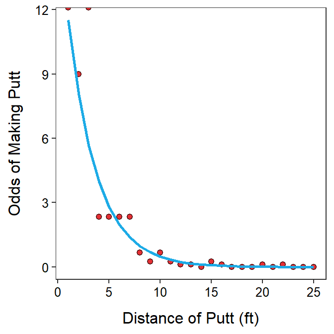
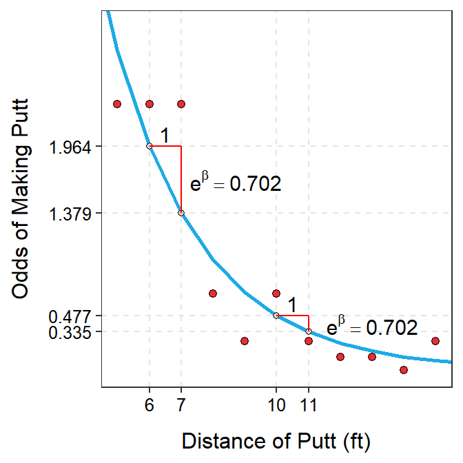
Figure 26.2: Odds of making a putt versus the distance of the putt with best-fit line superimposed. The right panel is ‘zoomed in’ on distances of 5 to 15 so that the exponentiated slope could be better seen.
Again, look closely at Figure 26.2-Right to understand the meaning of the exponentiated slope. When the distance of the putt increased from 6 to 7 feet the predicted odds declined from 1.964 to 1.379, a difference of 1.379-1.964= -0.585 but a ratio of \(\frac{1.379}{1.964}\)=0.702. When the distance of the putt was increased from 10 to 11 feet the difference in odds was 0.335-0.477= -0.142 but the ratio was \(\frac{0.335}{0.477}\), which was again 0.702. Thus, the difference in odds changes depending on the values of the explanatory variable but the ratio of odds stays constant at the value of the exponentiated slope (Table 26.2).
The exponentiated slope for a logistic regression is the multiplicative change in the odds for a unit change in the explanatory variable.
26.3 Predictions
The fitted logistic regression model can be used to make predictions. However, you must be very careful what is being predicted (i.e., the log odds) and how to back-transform (exponentiation gives the odds, not the probability).
Plugging a value of \(X\) into the fitted logistic regression equation will predict a value for the log odds. For example, the predicted log odds for making a 6 foot putt is 2.797-0.354×6 = 0.675 (values of α and β from Table 26.1 and log odds prediction shown in Figure 26.1).
Exponentiating this value results in the odds. Thus, the odds of making a 6 foot putt is e0.675=1.964 (Figure 26.2). Thus, the probability of making the 6 foot putt is nearly twice as likely as not making the 6 foot putt.
Finally, one most often wants to predict the probability of “success.” As shown in Module 25, a probability can be computed from the odds with \(p = \frac{\text{odds}}{\text{1+odds}}\). Thus, for example, the probability of making the 6 foot putt is \(\frac{1.964}{1+1.964}\)=0.663 (Figure 26.3). Therefore, the students makes a 6 foot put about 66% of the time on average (so, about 2 out of every 3).
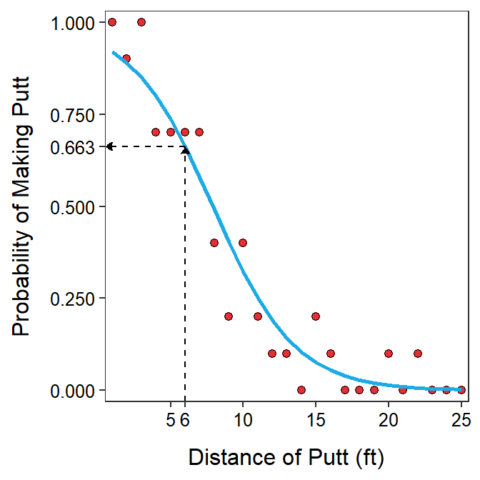
Figure 26.3: Probability of making a putt versus the distance of the putt with best-fit line superimposed and the prediction of the probability of making a 6 foot is shown.
26.4 “Reverse” Predictions
In logistic regression it is fairly common to ask a specific version of the generic question “What is the value of \(X\) for a given probability?” For example, one may be interested to determine the length of the putt where there is a 50% probability of making the putt. In other words, what is the distance when the probability of making the putt is no longer greater than the probability of not making the putt. Of course, one can consider other probabilities as well.
Solving the logistic regression equation for \(X\) provides an equation to answer these types of questions. The algebra to solve for \(X\) is shown below, beginning with the logistic regression equation.
\[ \begin{split} log\left(\frac{p}{1-p}\right) &= \alpha+\beta X \\ log\left(\frac{p}{1-p}\right)-\alpha &= \beta X \\ \beta X &= log\left(\frac{p}{1-p}\right)-\alpha \\ X &= \frac{log\left(\frac{p}{1-p}\right)-\alpha}{\beta} \\ \end{split} \]
For example, the distance for which the probability of making the putt is 0.1 is
\[ \frac{log\left(\frac{0.1}{1-0.1}\right)-2.797}{-0.354} = 14.12. \]
where values of α and β are from Table 26.1. This prediction is shown in Figure 26.4.
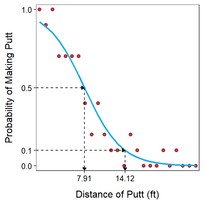
Figure 26.4: Probability of making a putt versus the distance of the putt with best-fit line superimposed and the prediction of the distances where the probabililty of making the putt is 0.10 and 0.50.
Because \(log(\left(\frac{0.5}{1-0.5}\right)\)=\(log(1)\)=0, the equation for predicting \(X\) for a given \(p\) reduces to \(X=\frac{-\alpha}{\beta}\) for \(p\)=0.5. Thus, the distance for which the probability of making the putt is 0.5 is 7.91 ft (Figure 26.4).
26.5 Another Example
As another example data about the presence or absence of a common shrub (Berberis repens) in the Bryce Canyon National Park Utah will be used. Here the researchers recorded whether the shrub was present or not in many 10m×10m plots throughout the park. They also recorded the elevation (among other things) of the plot. They wanted to model the effect of elevation on the presence of the shrub.
The estimated slope for the shrub data indicates that as the elevation increases by one meter, the log odds that the shrub is present increases by 0.0090 (95% CI: 0.0063, 0.0146; Table 26.3). The interpretation of the slope is made difficult by the fact that a 1 m change is a very small movement along the x-axis in this case where the elevations range from near 2000 to near 2800. However, if a 1 unit change in \(X\) results in an additive change in \(Y\) of the slope, then, for example, a 100 unit change in \(X\) results in an additive change in \(Y\) of 100 slopes. Thus, for example, if the elevation increases by 100 m then the log odds of the presence of the shrub will increase by 100×0.0090=0.90 (Figure 26.5).
| Ests | 2.5 % | 97.5 % | |
|---|---|---|---|
| (Intercept) | -21.6044 | -34.7819 | -15.3525 |
| elev | 0.0090 | 0.0063 | 0.0146 |
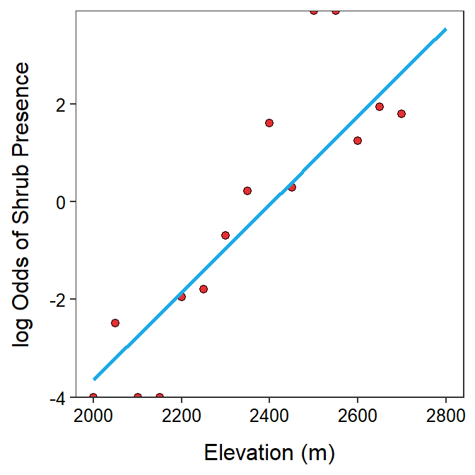
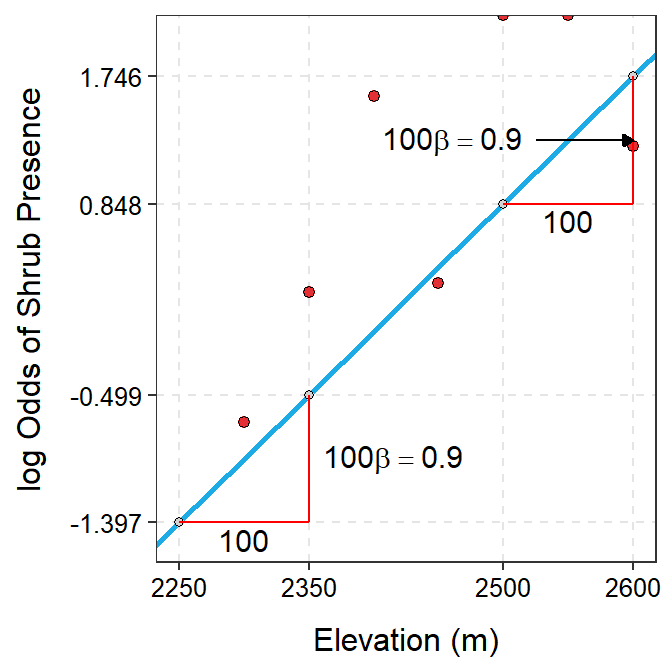
Figure 26.5: Log odds of shrub presence versus elevation with best-fit line superimposed. The right panel is ‘zoomed in’ on elevations of 2250 to 2600 m so that the slope could be better seen.
If a 1 unit change in \(X\) is very small relative to the range of \(X\) then multiplying the slope by an amount \(b\) will describe the additive change in the log odds for a \(b\) unit change in the explanatory variable.
The exponentiated estimated slope for the shrub data would have the same issue with scale described above for the estimated slope. The same remedy may be used but, as usual, you must be very careful with the interpretation. Exponentiating 100 times the slope suggests that as the elevation increases by 100 m, the odds that the shrub is present increases 2.455 (95% CI: 1.882, 4.289) times (Figure 26.6).
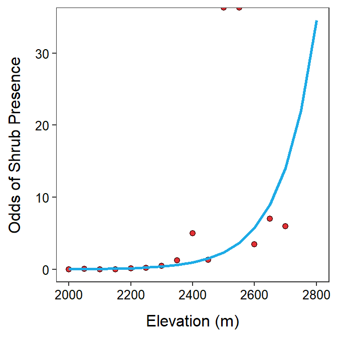
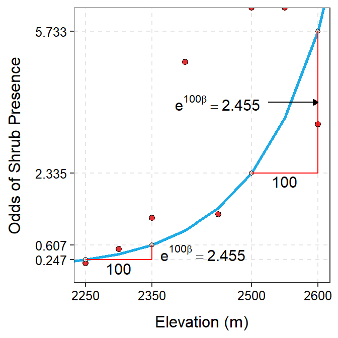
Figure 26.6: Odds of shrub presence versus elevation with best-fit line superimposed. The right panel is ‘zoomed in’ on elevations of 2250 to 2600 m so that the exponentiated slope could be better seen.
The exponentiated \(b\)×slope for a logistic regression is the multiplicative change in the odds for a \(b\) unit change in the explanatory variable.
The predicted log odds for the presence of the shrub at an elevation of 2350 m is -21.604+0.0090×2350 = -0.499 (values of α and β from Table 26.3 and log odds prediction shown in Figure 26.5). The odds of the shrub’s presence at an elevation of 2350 m is e-0.499=0.607 (Figure 26.6). Thus, the probability of the shrub being present at 2350 m is 0.607 times the probability that it is not present. Alternatively, the probability that the shrub is not present at 2350 m is 1.647 times the probability that it is present at that elevation (i.e., \(\frac{1}{0.607}\)). The probability that the shrub is present at 2350 m is 0.378 (=\(\frac{0.607}{1+0.607}\); Figure 26.7). Therefore, a little more than 1 out of every 3 plots at 2350 m will have the shrub.
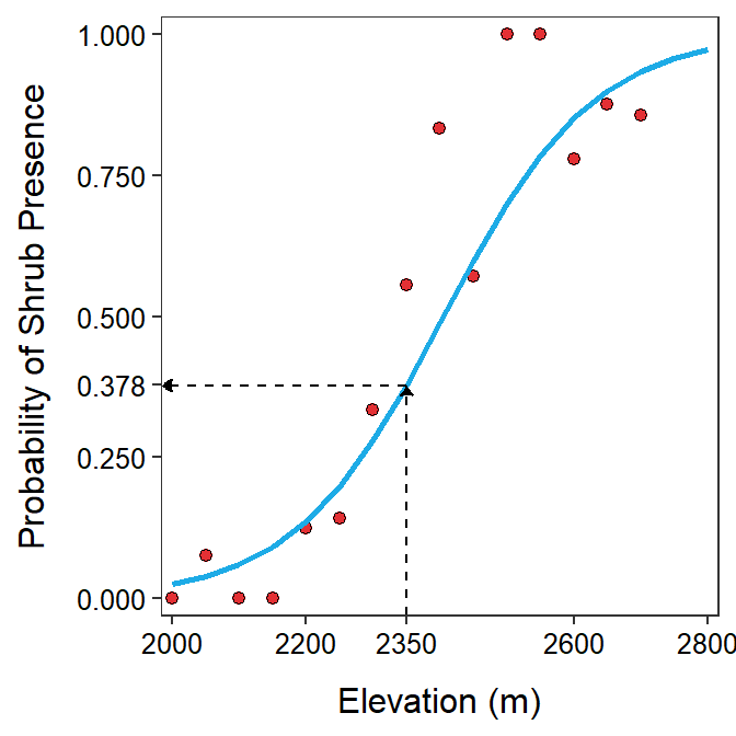
Figure 26.7: Probability of the shrub’s presence versus elevation with best-fit line superimposed and the prediction of the probability at 2350 m.
Finally, the elevation for which the probability of the shrub’s presence is 0.75 is
\[ \frac{log\left(\frac{0.95}{1-0.95}\right)--21.604}{0.0090} = 2733.4. \]
where values of α and β are from Table 26.3. Similarly, the elevation where there is an equal probability of the shrub being present or not is 2405.6 (=\(\frac{-(-21.604)}{0.0090}\)). These predictions are shown in Figure 26.8.
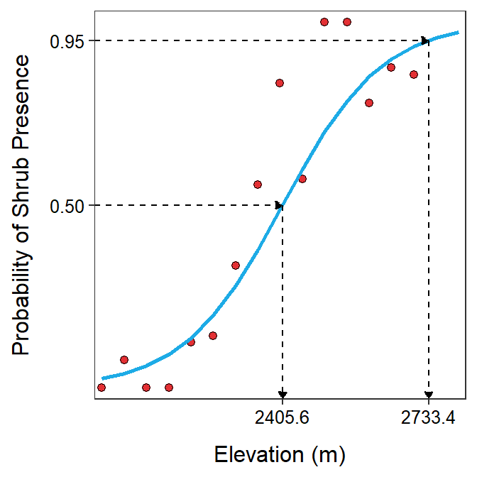
Figure 26.8: Probability of the shrub’s presence versus elevation with best-fit line superimposed and the prediction of elevations where the probabililty of the shrub’s presence is 0.50 and 0.75.
26.6 Variability Estimates
Standard errors or confidence intervals for the parameters of the logistic regression model can be computed with normal distribution theory. However, this theory does not hold for all logistic regression models. In addition, methods for computing confidence intervals for predicted probabilities or for predicted values of \(X\) for a particular probability are not well formed. Bootstrapping is one method for producing confidence intervals for these parameters.
Bootstrap confidence intervals are computer intensive, but provide an interval that does not depend on the shape of the underlying sampling distribution. Bootstrapping confidence intervals generally follows these steps:
- Generate a bootstrap sample, which is a random sample of individuals from the original sample;109
- Fit the model to the bootstrap sample;
- Compute the statistics of interest (i.e., the slope, intercept, predicted probability, predicted value of \(X\));
- Repeat steps 1-3 between 500 and10000 times;110
- Order the results from smallest to largest; and
- Approximate 95% confidence interval with the values of the statistics that have 2.5% and 97.5% of the statistics smaller (i.e., find the middle 95% of the bootstrapped statistics).111
A histogram of slopes estimated from 999 bootstrap samples is shown in Figure 26.9. It is apparent from this example that the sampling distribution of the slopes is not normal and, thus, a confidence interval generated from normal theory would not be appropriate. The 95% bootstrap confidence interval shown in Figure 26.9 matches that in Table 26.1.
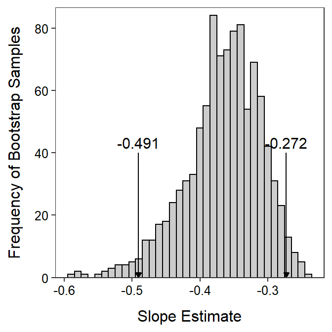
Figure 26.9: Histogram of logistic regression slopes from the golf putt example estimated from 999 bootstrap samples. The two values denoted mark the values with 2.5% and 97.5% of the slopes smaller and thus represents a 95% bootstrap confidence interval for the slope.
Bootstrapping is particularly useful for derived statistics like predicting the \(X\) for a given probability. A histogram of predicted distances where the probability of making the putt is 0.50 estimated from 999 bootstrap samples is shown in Figure 26.10. Thus, one is 95% confident that the distance of the putt where the probability of making the putt is 0.50 is between 6.86 and 8.95 feet.
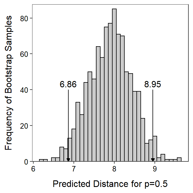
Figure 26.10: Histogram of the predicted distance where the probability making the putt is 0.50 estimated from 999 bootstrap samples. The two values denoted mark the values with 2.5% and 97.5% of the distances smaller and thus represents a 95% bootstrap confidence interval for the distance.
Actual construction of the bootstrap confidence intervals is illustrated in the next module.
The bootstrap method will be used to constructed confidence intervals for parameters in a logistic regression as typical normal theory is not always reliable with logistic regressions.
Thus, the individuals must be selected with replacement so that each bootstrap sample is different and different from the original sample.↩︎
The number of bootstrap samples depends on a number of things, including the purpose of the study and how involved the calculations are. In this course, 500-1000 bootstrap samples will be adequate.↩︎
This step tends to produce slightly biased results. There are a number of possible corrections for this bias. However, we will use this method in this course to keep the method simple so that we can stay focused on the concept.↩︎