Module 28 Logistic Regression Summary
Specific parts of a full Logistic Regression analysis were described in Modules 25-27. In this module, a workflow for a full analysis is offered and that workflow is demonstrated with an example.
28.1 Suggested Workflow
The following is a process for fitting a logistic regression. Consider this process as you learn to fit logistic regression models, but don’t consider this to be a concrete process for all models.
- Briefly introduce the study (i.e., provide some background for why this study is being conducted).
- State the hypotheses to be tested.
- Show the overall sample size.
- Address the independence assumption.
- If this assumption is not met then other analysis methods must be used.
- Fit the logistic regression module with
glm(). - Create a summary graphic of the fitted line with 95% confidence band using
ggplot(). Briefly assess if this model seems to fairly represent the raw data. - Perform a relationship test with
anova()to determine if the response and explanatory variables are significantly related. - Summarize findings with coefficient results and bootstrapped confidence intervals with
car::Boot()followed bycbind(coef(),confint()). Interpret the back-transformed slope (use the CI). - Demonstrate how the model can be used to predict the probability of a “success” given a value of the explanatory variable and the explanatory variable where the probability of success equals some value (usually 50%) (will use
predict(),predProb(),predX(), andquantile()). - Write a succinct conclusion of your findings.
28.2 Slimy Salamander Occurrence
A previous Biometry student examined the relationship between the presence/absence of Slimy Salamanders (Plethodon glutinosus) in counties from around the United States and the mean elevation of those same counties. Slimy Salamanders are generally thought to inhabit higher elevation areas and, thus, the student hypothesized that the probability for the presence of Slimy Salamanders would be higher in counties with higher mean elevations. To test this hypothesis the student gathered Slimy Salamander presence/absence data by county from the iNaturalist website. She then combined these data with other summary information, including mean elevation, from the same counties. Her database is in SlimySalamander.csv.
The statistical hypotheses to be examined are
\[ \begin{split} \text{H}_{\text{0}}&: ``\text{no relationship between the presence of Slimy Salamanders and the mean elevation of the county''} \\ \text{H}_{\text{A}}&: ``\text{is a relationship between the presence of Slimy Salamanders and the mean elevation of the county''} \\ \end{split} \]
Data were recorded for 1469 counties. The data between some counties may be related as both the elevation and presence of salamanders are probably similar for adjacent counties. However, given the exhaustive nature of the sample (the sample is most counties) these relations are unavoidable and likely mitigated by the large sample size. Thus, the independence assumption is not perfectly upheld, but it is also probably not problematic in this case.
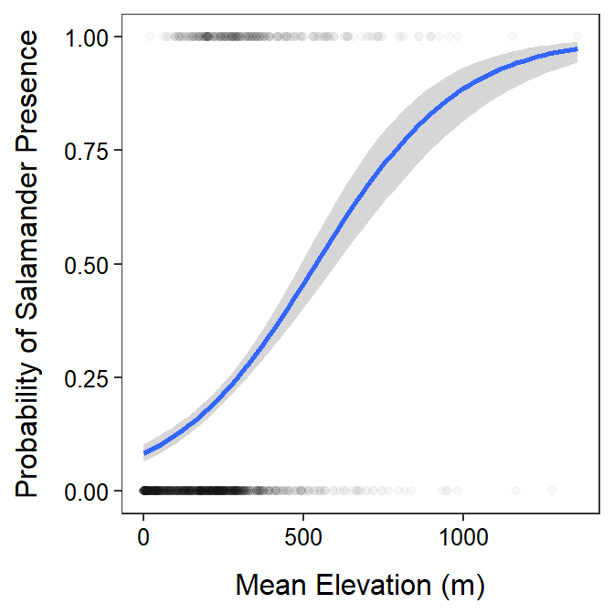
The are no specific assumptions to check in a binary logistic regression. However, the fitted line from the logistic regression (Figure 28.1) seems to at least capture the general trend of few counties at low elevations having Slimy Salamanders present with a general increase as the elevation increases. The model, however, is based on very few observations for elevations greater than about 500 m.

Figure 28.1: Best-fit logistic regression line and 95% confidence band for the probability of the presence of Slimy Salamanders in a county and the mean elevlation of the county.
The probability of Slimy Salamanders being present in a county appears to be significantly related to elevation of the county (LRT: p<0.00005; Table 28.1).
| Df | Deviance | Resid. Df | Resid. Dev | Pr(>Chi) | |
|---|---|---|---|---|---|
| NULL | 1468 | 1552.649 | |||
| elevation_m | 1 | 159.1 | 1467 | 1393.508 | 0 |
In fact it appears that the odds of a Slimy Salamander being present in the county is between 1.0036 and 1.0054 times greater for every 1 m increase in elevation (back-transformed slopes from Table 28.2). As 1 m is a very small increase in elevation, note that this translates to a 1.037 and 1.055 times increase in the odds of a Slimy Salamander being present for 10 m increase in elevation (these are the previous values raised to the 10th power). Thus, the odds of a Slimy Salamander being present is betwen 3.7% and 5.5% greater for every 10 m increase in elevation.
| Ests | 2.5 % | 97.5 % | |
|---|---|---|---|
| (Intercept) | -2.4136 | -2.6652 | -2.1951 |
| elevation_m | 0.0045 | 0.0036 | 0.0054 |
To demonstrate the utility of this model I made two predictions. First, the probability of the presence of Slimy Salamanders in a county with a mean elevation of 300 m is between 0.228 and 0.281. Second, the elevation where there is a 50% probability of Slimy Salamanders being present in the county is between 481 and 615.
In conclusion, a significantly positive relationship was found between the probability of Slimy Salamanders being found in a county and the mean elevation of the county. It appears that the student’s hypothesis about increasing presence of Slimy Salamanders with increasing elevation was upheld. In addition, the fitted model can be used to predict the probability of Slimy Salamander’s being present and the mean elevation at which that probability was 50%.
R Code and Results
predProb <- function(x,alpha,beta) exp(alpha+beta*x)/(1+exp(alpha+beta*x))
predX <- function(p,alpha,beta) (log(p/(1-p))-alpha)/beta

ss <- read.csv("https://raw.githubusercontent.com/droglenc/Book207/main/docs/data/SlimySalamanders.csv")
logreg <- glm(salamander_presence~elevation_m,data=ss,family=binomial)

anova(logreg,test="LRT")
b_logreg <- car::Boot(logreg)
cfs <- cbind(Ests=coef(logreg),confint(b_logreg,type="perc"))
p_prob <- predProb(300,b_logreg$t[,1],b_logreg$t[,2])
ci_prob <- quantile(p_prob,c(0.025,0.975),type=1)
p_x <- predX(0.50,b_logreg$t[,1],b_logreg$t[,2])
ci_x <- quantile(p_x,c(0.025,0.975),type=1)

ggplot(data=ss,mapping=aes(x=elevation_m,y=salamander_presence)) +
  geom_point(alpha=0.025) +
  geom_smooth(method="glm",method.args=list(family=binomial)) +
  labs(x="Mean Elevation (m)",
       y="Probability of Salamander Presence") +
  theme_NCStats()