Module 23 IVR Analysis

Modules 20-22 built a conceptual and analytical foundation for an indicator variable regresion (IVR). Three more analytical topics need to be addressed before a full IVR can be completed in Module 24. Those topics – assumptions and transformations, multiple comparisons for slopes, and multiple comparisons for intercepts – are introduced in this module.

23.1 Assumptions & Transformations

The assumptions for an IVR are the same as those for an SLR – independence, linearity, homoscedasticity, normality, and no outliers (see Module 17). Methods for assessing the validity of these assumptions are also essentially the same as those used for an SLR. In other words, residual plots will be used to examine linearity and assess homoscedasticity, an Anderson-Darling test and a histogram of the residuals will be used to assess the normality of residuals, and a residual plot and an outlier test will be used to diagnose outliers and influential points.

An important point to note, though, is that the IVR assumptions are assessed on the ultimate full model. If the assumptions are not met on the ultimate full model, then transformations for the response and the covariate⁹⁹ should be considered such that a transformed version of the ultimate full model meets the assumptions.¹⁰⁰ Once an ultimate full model is found where all assumptions are met, then it is assumed that all assumptions will be met for any subset of the ultimate full model that has non-significant explanatory variables removed.

The assumptions of an IVR are the same as the assumptions for an SLR. Thus, methods for assessing the assumptions are the same as those methods used for an SLR

IVR assumptions are assessed for the ultimate full model. Assumptions do not need to be assessed for simpler models that only have variables from the ultimate full model removed.

23.2 Multiple Comparisons for Slopes

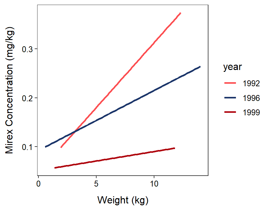
In Section 22.6, IVR indicated that some slopes between mirex concentration in the tissue and salmon weight differed among 1992, 1996, and 1999 (Figure 23.1). An examination of Figure 23.1 suggests that the slopes for 1992, 1996, and 1999 are all likely not the same. However, an objective method is needed to determine which pairs of slopes actually differ. Parallel lines tests for IVRs taking two years at a time could be used but this is inefficient and would increase the experiment-wise error rate (recall from Section 6.1).

 

Figure 23.1: Fitted regression lines for mirex in tissue by salmon weight for 1992, 1996, and 1999. Note that the IVR indicated that these lines are not parallel.

 

The emtrends() function from the emmeans package¹⁰¹ can be used to test for differences among all pairs of slopes using a Tukey-like correction. This function requires the ultimate full model as its first argument (ivrY1 here as fit in Section 22.2), a specs= argument with pairwise~ followed by the name of the factor variable in the ultimate full model, and var= followed by the name of the covariate in the ultimate full model (which must be in quotes).¹⁰² The results of this function should be saved to an object.

smc <- emtrends(ivrY1,pairwise~year,var="weight")

That saved object is then the first argument to summary(), which also includes infer=TRUE. The results are in sections labeled as $emtrends and $contrasts.

( smcsum <- summary(smc,infer=TRUE) )

#R>  $emtrends
#R>   year weight.trend      SE df lower.CL upper.CL t.ratio p.value
#R>   1992      0.02653 0.00483 44  0.01679   0.0363   5.489  <.0001
#R>   1996      0.01225 0.00306 44  0.00609   0.0184   4.004  0.0002
#R>   1999      0.00386 0.00499 44 -0.00620   0.0139   0.773  0.4434
#R>  
#R>  Confidence level used: 0.95 
#R>  
#R>  $contrasts
#R>   contrast    estimate      SE df  lower.CL upper.CL t.ratio p.value
#R>   1992 - 1996  0.01428 0.00572 44  0.000403   0.0282   2.496  0.0425
#R>   1992 - 1999  0.02267 0.00695 44  0.005815   0.0395   3.262  0.0059
#R>   1996 - 1999  0.00839 0.00586 44 -0.005813   0.0226   1.433  0.3331
#R>  
#R>  Confidence level used: 0.95 
#R>  Conf-level adjustment: tukey method for comparing a family of 3 estimates 
#R>  P value adjustment: tukey method for comparing a family of 3 estimates

The $contrasts section contains the Tukey-corrected tests for each pair of slopes. The important columns in these results are

• estimate: the difference in group sample slopes,
• lower.CL and upper.CL: 95% confidence interval for the difference in slopes, and
• p.value: p-value for testing that the difference in slopes is 0 or not.

For example, the sample slope for 1992 is 0.01428 greater than the sample slope for 1996, one is 95% confident that the population slope for 1992 is between 0.000403 and 0.0282 greater than the population slope for 1996, and the population slopes differ between 1992 and 1996 (p=0.0425). In contrast, the sample slope for 1996 is 0.00839 greater than the sample slope for 1999, one is 95% confident that the population slope for 1996 is between 0.005813 less than and 0.0226 greater than the population slope for 1999, and the population slopes do NOT differ between these two years (p=0.3331).

An examination of all of the $contrast results suggests that the slope from 1992 differed significantly from the slopes of 1996 (p=0.0425) and 1999 (p=0.0059), but the slopes for 1996 and 1999 did not differ (p=0.3331).

The difference in group slopes with 95% confidence intervals and p-values are shown in the $contrasts section of the results.

The $emtrends section of the output contains information about the individual slopes, specifically.

• XXX.trend: the sample slope (note that XXX will be replaced with the name of the covariate in the model),
• lower.CL and upper.CL: 95% confidence interval for the slope, and
• p.value: p-value for the test whether the slope is 0 or not (i.e., is there a relationship or not).

For example, the sample slope for 1992 is 0.02653, one is 95% confident that the population slope for 1992 is between 0.01679 and 0.0363, and there is a significant relationship between mirex in the tissue and salmon weight in 1992 (p<0.00005).

An examination of all of the results in $emtrends shows that the only slope that was not significantly different from 0 was for 1999. Thus, there was a significant relationship between mirex concentration in the tissue and salmon weight for 1992 and 1996, but not for 1999.

The slopes with 95% confidence intervals and p-values for testing if the slope is 0 or not are shown in the $emtrends section of the results.

23.3 Multiple Comparisons for Intercepts

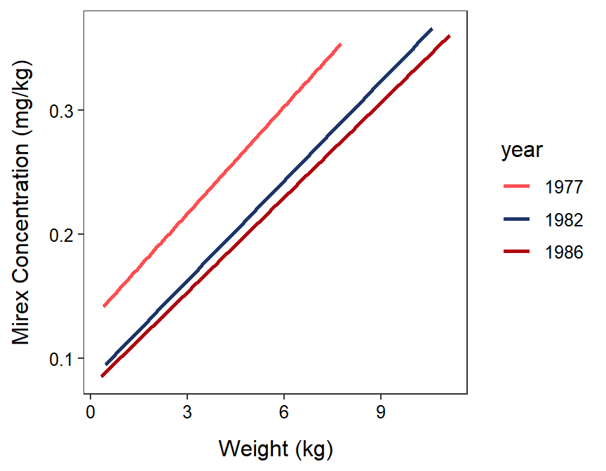
In Section 22.7 of the last module, the IVR indicated that the first three years (1977, 1982, and 1986) had the same slopes and that at least some of those years had different intercepts (Figure 23.2).¹⁰³ An examination of Figure 23.2 suggests that the intercept for 1977 may be greater than the intercepts for 1982 and 1986, which likely do not differ significantly. Again, an objective method is needed to determine which pairs of intercepts significantly differ.

 

Figure 23.2: Fitted regression lines for mirex in tissue by salmon weight for only 1977, 1982, and 1986. Note that the IVR indicated that these lines are parallel, there is a signficant relationship, and at least one of the lines has a different intercept.

 

The emmeans() function from the emmeans package can be used to determine which pairs of intercepts differ (using a Tukey’s correction). However, before using this function a new model with the insignificant interaction term removed should be fit.

ivrY2_noint <- lm(mirex~weight+year,data=MirexFirst3)

The use of emmeans() here is exactly the same as it was in Section 6.3. Specifically, the model without the interaction term is the first argument and pairwise~ is followed by the name of the factor variable in the model. The results are then submitted to summary() with infer=TRUE and the results are given in two sections labeled $emmeans and $contrasts.

imc <- emmeans(ivrY2_noint,pairwise~year)
( imcsum <- summary(imc,infer=TRUE) )

#R>  $emmeans
#R>   year emmean     SE df lower.CL upper.CL t.ratio p.value
#R>   1977  0.238 0.0123 68    0.213    0.262  19.392  <.0001
#R>   1982  0.184 0.0122 68    0.159    0.208  15.091  <.0001
#R>   1986  0.172 0.0123 68    0.148    0.197  14.015  <.0001
#R>  
#R>  Confidence level used: 0.95 
#R>  
#R>  $contrasts
#R>   contrast    estimate     SE df lower.CL upper.CL t.ratio p.value
#R>   1977 - 1982   0.0542 0.0173 68   0.0128   0.0956   3.139  0.0070
#R>   1977 - 1986   0.0655 0.0175 68   0.0235   0.1075   3.736  0.0011
#R>   1982 - 1986   0.0113 0.0173 68  -0.0302   0.0529   0.653  0.7913
#R>  
#R>  Confidence level used: 0.95 
#R>  Conf-level adjustment: tukey method for comparing a family of 3 estimates 
#R>  P value adjustment: tukey method for comparing a family of 3 estimates

The important parts of the $contrasts portion are

• estimate: the difference in sample intercepts,
• lower.CL and upper.CL: 95% confidence intervals for the difference in intercepts, and
• p.value: p-value for whether the differences in intercepts is 0 or not.

For example, the sample intercept for 1977 is 0.0542 mg/kg greater than the intercept for 1982, the population intercept for 1977 is between 0.0128 and 0.0956 greater than the population intercept for 1982, and the intercepts for these two years are significantly different (p=0.0070). Because these two years are parallel, the sample mean mirex concentration for 1977 is 0.0542 mg/kg greater than the sample mean mirex concentration for 1982 for all salmon weights.

The difference in group intercepts with 95% confidence intervals and p-values are shown in the $contrasts section of the results.

The results in the $emmeans portion contains information about the mean of the response variable at the mean of the covariate. In other words, this information is about the intercepts for the centered covariate (see Section 15.3). Specifically,

• emmean: sample mean of the response variable at the sample mean of the covariate,
• lower.CL and upper.CL: 95% confidence interval for the population mean of the response variable at the sample mean of the covariate, and
• p.value: a p-value for testing if the population mean of the response variable at the sample mean of the covariate is equal to 0 or not.

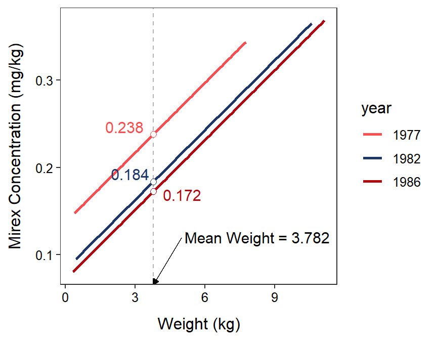
For example, the sample mean mirex concentration in 1977 for salmon with the sample mean weight of all salmon is 0.238, one is 95% confident that the population mean mirex concentration in 1977 for a salmon with the sample mean weight of all salmon is between 0.213 and 0.262 mg/kg, and the population mean mirex concentration at the sample mean salmon weight in 1977 is not equal to 0 (p<0.00005). A visual of the sample means under emmeans is shown in Figure 23.3.

 

Figure 23.3: Fitted regression lines for mirex in tissue by salmon weight for only 1977, 1982, and 1986. The mean mirex concentration at the mean salmon weight is shown for each year to demonstrate the results of the emmeans() function.

 

The mean value of the response at the mean value of the covariate, along with 95% confidence intervals and p-values, are shown in the $emmeans section of the results.

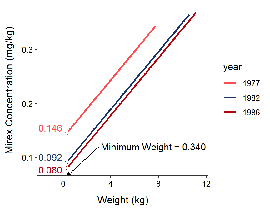
The emmeans() function defaults to showing the mean value of the response for the mean value of the covariate because the intercept is often an extrapolation as discussed in Section 15.3. It is possible to compute the mean values of the response at other values of the covariate by using cov.reduce= in emmeans(). For example, the code below computes the mean values of the response at the minimum value of the covariate (and shown in Figure 23.4).¹⁰⁴ Because the lines are parallel this does not change anything in the $contrasts portion of the output. However, the $emmeans portion is changed because the mean values of the response is computed at, in this example, the minimum value rather than the mean value of the covariate. Using the default calculation at the mean of covariate is probably most appropriate for most situations in general and all situations in this course.

imc2 <- emmeans(ivrY2_noint,pairwise~year,cov.reduce=min)
( imc2sum <- summary(imc2,infer=TRUE) )

#R>  $emmeans
#R>   year emmean     SE df lower.CL upper.CL t.ratio p.value
#R>   1977 0.1460 0.0143 68   0.1174    0.175  10.181  <.0001
#R>   1982 0.0918 0.0151 68   0.0617    0.122   6.097  <.0001
#R>   1986 0.0805 0.0163 68   0.0479    0.113   4.928  <.0001
#R>  
#R>  Confidence level used: 0.95 
#R>  
#R>  $contrasts
#R>   contrast    estimate     SE df lower.CL upper.CL t.ratio p.value
#R>   1977 - 1982   0.0542 0.0173 68   0.0128   0.0956   3.139  0.0070
#R>   1977 - 1986   0.0655 0.0175 68   0.0235   0.1075   3.736  0.0011
#R>   1982 - 1986   0.0113 0.0173 68  -0.0302   0.0529   0.653  0.7913
#R>  
#R>  Confidence level used: 0.95 
#R>  Conf-level adjustment: tukey method for comparing a family of 3 estimates 
#R>  P value adjustment: tukey method for comparing a family of 3 estimates

 

Figure 23.4: Fitted regression lines for mirex in tissue by salmon weight for only 1977, 1982, and 1986. The mean mirex concentration at the MINIMUM salmon weight is shown for each year to demonstrate the results of the emmeans() function.

 

---

99. If the covariate is transformed then any interaction terms with the covariate should be recreated using the transformed covariate.↩︎

100. The methods and rules for transforming these variables in an IVR are the same as those used for an SLR (see 18).↩︎

101. The emmeans package was introduced in Section 6.3.↩︎

102. Except for var= this is the same as for emmeans() described in Section 6.3↩︎

103. Recall from last module that those three years were chosen simply to serve as an example. Choosing these years has nothing to do with the analysis from the previous section.↩︎

104. You can get the mean values of the response at a covariate of 0 (i.e., the actual y-intercepts) by using cov.reduce=function(x) 0.↩︎