Module 22 IVR Testing
Hypothesis testing in an Indicator Variable Regression (IVR) is the same as that for the three previous methods, but it can feel different. Fortunately, this is where all of your hard work with respect to comparing models is going to pay off. Lets revisit the F-ratio test statistic (from Section 4.6) before discussing three specific hypotheses of an IVR.
22.1 F-ratio Test Statistic
The F-ratio test statistic was \(\text{F}=\frac{\text{MS}_{\text{Among}}}{\text{MS}_{\text{Within}}}\) for a One-Way ANOVA, the same for a Two-Way ANOVA except that MSAmong was replaced with MSA, MSB, or MSA:B, and was \(\text{F}=\frac{\text{MS}_{\text{Regression}}}{\text{MS}_{\text{Residual}}}\) for SLR. While these F-ratios all have different symbols they are all have this same general format:
\[ \text{F}=\frac{\text{Variance EXPLAINED by the full model}}{\text{Variance UNEXPLAINED by the ultimate full model}}=\frac{``\text{Signal''}}{``\text{Noise''}} \]
Note that the “noise” is always the residual MS from fitting the ultimate full model. In other words, the “noise” is the unexplained variance after ALL explanatory variables have been considered.
The “signal” or variance explained by the full model (that is not explained by the simple model) is a bit tricky with an IVR because what exactly the simple and full models are depends on the hypotheses being tested. These hypotheses and models are discussed in the next three sections. However, the variance explained by the full model is simply the difference in lack-of-fit between the two models divided by the difference in number of parameters between the two models. This is the “benefit-to-cost” ratio from Section 4.6 and is generically
\[ ``\text{Signal''}=\frac{\text{RSS}_{\text{Simple}}-\text{RSS}_{\text{Full}}}{\text{df}_{\text{Simple}}-\text{df}_{\text{Full}}} = \frac{``\text{Benefit (decrease in lack-of fit)''}}{``\text{Cost (increase in parameters)''}} \]
This means that the generic F-ratio test statistic is
\[ \text{F}=\frac{``\text{Signal''}}{``\text{Noise''}}=\frac{\frac{\text{RSS}_{\text{Simple}}-\text{RSS}_{\text{Full}}}{\text{df}_{\text{Simple}}-\text{df}_{\text{Full}}}}{\text{RMS}_{\text{Ultimate Full}}} \]
This formula will be applied in the next three sections.
22.2 Parallel Lines Test
Testing if groups have the same relationship between the response variable and the covariate is a common and important question. For example, one may ask if the relationship between mirex concentration and weight is the same for Coho and Chinook Salmon. Be clear, this is not asking if mirex concentration is the same for Coho and Chinook Salmon, rather it is asking if the relationship or rate of change of mirex concentration relative to weight is the same between the two species. Mirex concentrations may be higher or lower in Coho than Chinook, but here the question is if mirex changes at the same rate or not for the two species.
Asking if the relationship is the same among groups is the same as asking if the slopes are the same among groups, which is the same as asking if the lines are parallel. Thus, the test for answering this question is is called a parallel lines test.
In words, the hypotheses for a parallel lines test are
\[ \begin{split} \text{H}_{\text{0}}&: ``\text{The Coho and Chinook lines are parallel''} \\ \text{H}_{\text{A}}&: ``\text{The Coho and Chinook lines are NOT parallel''} \\ \end{split} \]
More usefully these translate into the following models96
\[ \begin{split} \text{H}_{\text{0}}&: \mu_{MIREX|\cdots} = \alpha+\beta WEIGHT+\delta_{1}COHO \\ \text{H}_{\text{A}}&: \mu_{MIREX|\cdots} = \alpha+\beta WEIGHT+\delta_{1}COHO+\gamma_{1}WEIGHT:COHO \\ \end{split} \]
Take note that HA includes the interaction term, whereas H0 does not. Recall from Section 21.3 that coefficients on the interaction terms correspond to differences in slopes. The H0 without this parameter corresponds to lines that are parallel, whereas HA with this parameter corresponds to lines with different slopes (and, thus, lines that are not parallel; Figure 22.1).
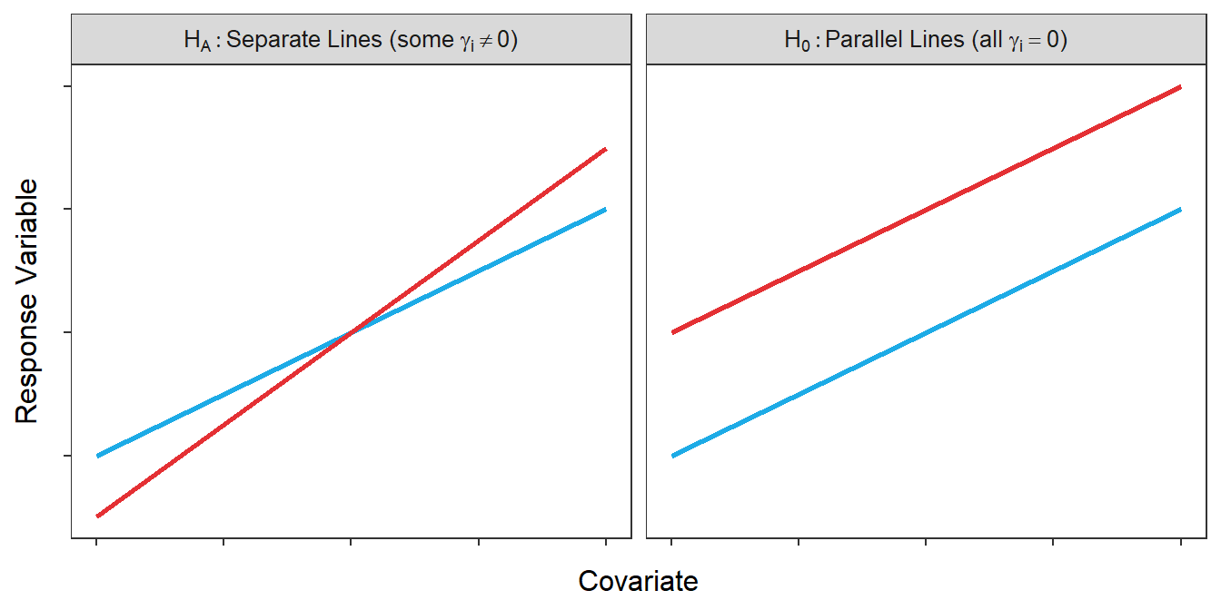
Figure 22.1: Hypothetical depictions of the models for the null and alternative hypotheses of the parallel lines test.
Parallel Lines Test: An F test to determine if all groups in an IVR can be described by lines with the same slope.
A parallel lines test is conducted by comparing the ultimate full model to the model that contains only the covariate and indicator variables (i.e., no interaction variables with the quantitative variable are included).
Parallel Lines Test from Two Models in R
The ultimate full model provides the residual MS for the F-ratio and also serves as the full model for the parallel lines test. The ultimate full model was fit in Section 21.4 as
ivr1 <- lm(mirex~weight+species+weight:species,data=Mirex)The simple model for the parallel lines test is the ultimate full model without the interaction variable(s).
ivr2 <- lm(mirex~weight+species,data=Mirex)The comparison of the simple and full models can be summarized by submitting the two models to anova() (simple model first).
anova(ivr2,ivr1)#R> Analysis of Variance Table
#R>
#R> Model 1: mirex ~ weight + species
#R> Model 2: mirex ~ weight + species + weight:species
#R> Res.Df RSS Df Sum of Sq F Pr(>F)
#R> 1 119 1.00708
#R> 2 118 0.97964 1 0.027444 3.3057 0.07158The first two columns of these results (Res.Df and RSS) are the residual df and RSS for each model (the simple model is listed first). As the full model here is also the ultimate full model, the residual MS for the denominator (bottom part) of the F-ratio is computed from the second row of these two columns. The next two columns (Df and Sum of Sq) are the differences between the residual df and SS of the two models; thus, these columns contain the two parts needed for the numerator (top part) of the F-Ratio. Thus, the F-ratio is computed with
\[ \text{F}=\frac{\frac{\text{RSS}_{\text{Simple}}-\text{RSS}_{\text{Full}}}{\text{df}_{\text{Simple}}-\text{df}_{\text{Full}}}}{\text{RMS}_{\text{Ultimate Full}}} =\frac{\frac{1.00708-0.97964}{119-118}}{\frac{0.97964}{118}} = \frac{\frac{0.027444}{1}}{0.00830} = \frac{0.02744}{0.00830} = 3.30566 \]
This calculation is the same (within rounding) as the value under F in the anova() results. The corresponding p-value is under the Pr(>F) column.
This p-value is larger than our typical rejection level of 0.05. Thus, we conclude that H0 is NOT rejected, the simple model is adequate (as compared to the full model), the slopes appear to be equal, and the lines are parallel. With parallel lines, one concludes that the relationship between mirex concentration in the tissue and weight of the salmon is the same for Coho and Chinook Salmon.
Two other hypothesis tests are considered in the next two sections. However, note that the parallel lines test is always considered first, because it is basically testing for an interaction effect. Thus, if the lines are not parallel (i.e., there is an interaction effect) then you will not perform the tests in the next two sections. Note that this is exactly what you did with the Two-Way ANOVA, where the significance of the interaction effect was assessed first, before deciding whether main effects could be considered.
The parallel lines test is ALWAYS conducted first as it involves the interaction variable(s).
22.3 Coincident Lines Test
If the groups are found to be parallel (i.e., have equal slopes) then you should proceed to determine if the groups also have equal intercepts. If the lines are both parallel and have equal intercepts then they are the same line, or are coincident. Thus, this test is called the coincident lines test.
In words, the hypotheses for a coincident lines test are
\[ \begin{split} \text{H}_{\text{0}}&: ``\text{Coho and Chinook lines are coincident''} \\ \text{H}_{\text{A}}&: ``\text{Coho and Chinook lines are parallel but not coincident''} \\ \end{split} \]
More usefully these translate into the following models
\[ \begin{split} \text{H}_{\text{0}}&: \mu_{MIREX|\cdots} = \alpha+\beta WEIGHT \\ \text{H}_{\text{A}}&: \mu_{MIREX|\cdots} = \alpha+\beta WEIGHT+\delta_{1}COHO \\ \end{split} \]
There are several important things to consider here. First, HA here was H0 in the parallel lines test. This illustrates that whether a model is a full or a simple model may depend on the hypothesis being tested. Second, interaction variables are not present in either model because the coincident lines test is only considered for parallel lines (and, thus, the interaction term depicting the difference in slopes is not included). Third, the difference between the two models is the inclusion of the indicator variable and its \(\delta_{i}\) coefficient. Recall from Section 21.3 that \(\delta_{i}\) measures the differences in intercepts. The H0 without this parameter (and without \(\gamma_{i}\)) corresponds to lines that are exactly the same, whereas HA with this parameter corresponds to some lines that have different intercepts (but the same slope; Figure 22.2).
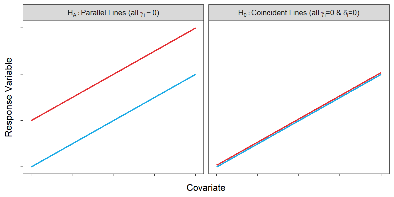
Figure 22.2: Hypothetical depictions of the models for the null and alternative hypotheses of the coincident lines test.
This needs to be very clear – the coincident lines test is relevant only if the lines have already been found to be parallel. Thus, you will only test for equal intercepts AFTER having already determined that the lines are parallel. If the lines are not parallel then you will NOT conduct a coincident lines test. The reasoning for this can be thought of in at least two ways.
First, differences in intercepts come from examining the indicator variable(s). The indicator variables stem from one original factor variable and, thus, can be thought of as a “main effect.” If the parallel lines test indicates non-parallel lines then a significant interaction has been found to be an important contributor to the model. As was learned with a two-way ANOVA, if an interaction exists in the model then the main effects should not be interpreted.
Second, if the lines are not parallel then the significance of the intercept term depends on the relative magnitude of the slopes and “how far” the observed data is from \(X=0\). For example, the intercepts in Figure 22.3-Left are statistically different. However, if the center of the observed data was on \(X=0\) as in Figure 22.3-Right then the intercepts would not be statistically different. In summary, the test for equal intercepts is not useful if the slopes differ between groups.
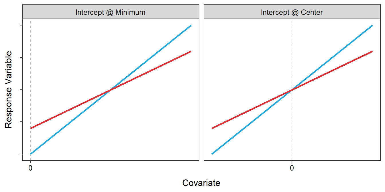
Figure 22.3: Representation of two sub-model fits with non-parallel lines. The left plot illustrates a situation where X=0 is at the left margin of the observed data. The right plot illustrates a situation where X=0 is at the center of the observed data. Overall, the two plots illustrate how the difference in intercepts depends on where X=0 is relative to the two fitted lines.
On the other hand, if the lines are parallel then the coincident lines test is very important. With parallel lines the difference in intercepts is a measure of the vertical difference between the lines for every value of the covariate. Thus, the difference in intercepts is a measure of the difference in the response variable between the groups at the same value of the covariate. The coincident lines test tests whether this constant difference is significantly different than 0 or not. In other words, do the values of \(Y\) for each group differ for each value of \(X\).
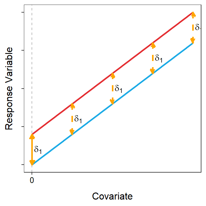
Figure 22.4: Representation of two sub-model fits that are parallel but with different intercepts (not coincident). The difference in intercepts is shown at X=0, but since the lines are parallel this is the same difference at every value of X, four others of which are shown.
Coincident Lines Test: An F test to determine if all groups in an IVR can be described by lines with the same intercept given that the lines have equal slopes.
A coincident lines test is only appropriate if the lines are parallel.
The coincident lines test (assuming parallel lines) tests whether the mean of the response variable differs between groups for all values of covariate.
Coincident Lines Test from Two Models in R
The full model for the coincident lines test was the simple model for the parallel lines test and was fit previously and saved as ivr2. The simple model for the coincident lines test is the simple linear regression model (i.e., no difference in slopes or intercepts); i.e.,
ivr3 <- lm(mirex~weight,data=Mirex)These models are compared with anova(); however, the ultimate full model must be included as well so that the proper residual MS (i.e., from the ultimate full model) will be used.
anova(ivr3,ivr2,ivr1)#R> Analysis of Variance Table
#R>
#R> Model 1: mirex ~ weight
#R> Model 2: mirex ~ weight + species
#R> Model 3: mirex ~ weight + species + weight:species
#R> Res.Df RSS Df Sum of Sq F Pr(>F)
#R> 1 120 1.00758
#R> 2 119 1.00708 1 0.0004983 0.0600 0.80690
#R> 3 118 0.97964 1 0.0274436 3.3057 0.07158These results are organized similar to before, but we can focus on the first two rows as RMSUltimate Full was calculated previously when completing the parallel lines test. Thus, the F-ratio is calculated with
\[ \text{F}=\frac{\frac{\text{RSS}_{\text{Simple}}-\text{RSS}_{\text{Full}}}{\text{df}_{\text{Simple}}-\text{df}_{\text{Full}}}}{\text{RMS}_{\text{Ultimate Full}}} =\frac{\frac{1.00758-1.00708}{120-119}}{0.00830} = \frac{\frac{0.00050}{1}}{0.00830} = \frac{0.00050}{0.00830} = 0.06002 \]
Again, this is the F test-statistic (within rounding) shown in the (second row of the) anova() results.
This p-value (p=0.8087) is larger than our typical rejection level of 0.05. Thus, we conclude that H0 is NOT rejected, the simple model is adequate (as compared to the full model), the intercepts appear to be equal, and the lines are coincident. With coincident lines, one can conclude, in addition to the relationship not differing between groups (i.e., parallel lines), that the mean mirex concentration in the tissue does NOT differ between Coho and Chinook Salmon of the same weight, no matter what that weight is.
22.4 Relationship Test
If the lines are found to be parallel then you should also determine if the lines represent a relationship or not. This reduces to determining if the slope of the reference group is different from zero (a flat line) or not (not a flat line). As the lines are parallel, the decision for the reference group will extend to the other groups.
In words, the hypotheses for the relationship test are
\[ \begin{split} \text{H}_{\text{0}}&: ``\text{There is no relationship between mirex and weight''} \\ \text{H}_{\text{A}}&: ``\text{There is a relationship between mirex and weight (for the coincident lines)''} \\ \end{split} \]
More usefully these translate into the following models
\[ \begin{split} \text{H}_{\text{0}}&: \mu_{MIREX|\cdots} = \alpha \\ \text{H}_{\text{A}}&: \mu_{MIREX|\cdots} = \alpha+\beta WEIGHT \\ \end{split} \]
At first glance, this appears to be the same models used in an SLR (Figure 22.5). However, in an IVR, the denominator in the F-ratio is from the ultimate full model. Therefore, the measure of “noise” in an IVR considers more variables than are considered in an SLR. Thus, the conclusion could differ between a relationship test in an IVR and the similar looking SLR.
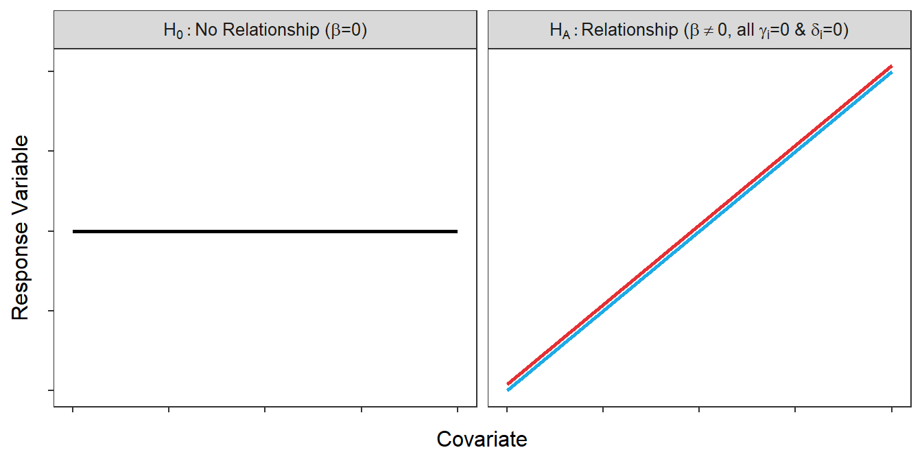
Figure 22.5: Hypothetical depictions of the models for the null and alternative hypotheses of the relationships test.
Notice in these models that the full model in the relationship test is the same as the simple model in the coincident lines test. Thus, the relationship test follows a coincident lines test. However, the relationship test can be conducted and interpreted regardless of the outcome of the coincident lines test.
The relationship test should, however, only be conducted if the lines are found to be parallel. The relationship test is concerned solely with the covariate and, thus, can be thought of as a “main effect,” which should only be considered in the absence of an interaction effect (i.e., parallel lines). Additionally, if the lines are not parallel that means the relationship between the response and covariate differs among groups and there is not one relationship to describe, as the relationship test attempts to do.
Relationship Test:: An F test to determine if a relationship exists between the response variable and the covariate in an IVR given that the lines are parallel.
A relationship test is only appropriate if the lines are parallel.
Relationship Test from Two Models in R
The full model for the relationship test was the simple module for the coincident lines test and was fit previously and saved as ivr3. The simple model for the relationship test is the so-called ultimate simple model97 and is fit with
ivr4 <- lm(mirex~1,data=Mirex)These models are compared with anova(), again with the ultimate full model included so that the proper residual MS will be used.
anova(ivr4,ivr3,ivr1)#R> Analysis of Variance Table
#R>
#R> Model 1: mirex ~ 1
#R> Model 2: mirex ~ weight
#R> Model 3: mirex ~ weight + species + weight:species
#R> Res.Df RSS Df Sum of Sq F Pr(>F)
#R> 1 121 1.23056
#R> 2 120 1.00758 1 0.222980 26.8586 9.155e-07
#R> 3 118 0.97964 2 0.027942 1.6828 0.1903These results are organized similar to before; thus, the F-ratio is calculated with
\[ \text{F}=\frac{\frac{\text{RSS}_{\text{Simple}}-\text{RSS}_{\text{Full}}}{\text{df}_{\text{Simple}}-\text{df}_{\text{Full}}}}{\text{RMS}_{\text{Ultimate Full}}} =\frac{\frac{1.23056-1.00758}{121-120}}{0.00830} = \frac{\frac{0.22298}{1}}{0.00830} = \frac{0.22298}{0.00830} = 26.8586 \]
Again, this is the F test-statistic (within rounding) shown in the (second row of the) anova() results.
This p-value (p<0.00005) is less than our typical rejection level of 0.05. Thus, one would conclude that H0 is rejected, the simple model is not adequate and the full model is needed, the slope for the coincident lines is not 0, and there is a relationship between mirex in the tissue and the weight of the salmon.
22.5 All Tests in R
The parallel lines, coincident lines, and relationship tests of an IVR appears to require fitting four models as shown in the previous three sections. However, these tests can be calculated more succinctly by submitting ONLY the ultimate full model (i.e., ivr1) to anova().
anova(ivr1)#R> Analysis of Variance Table
#R>
#R> Response: mirex
#R> Df Sum Sq Mean Sq F value Pr(>F)
#R> weight 1 0.22298 0.222980 26.8586 9.155e-07
#R> species 1 0.00050 0.000498 0.0600 0.80690
#R> weight:species 1 0.02744 0.027444 3.3057 0.07158
#R> Residuals 118 0.97964 0.008302A close comparison of this one set of results to the results in the three previous sections shows that
- The
weight:species(i.e., the interaction variable) row corresponds to the parallel lines test. - The
species(i.e., the factor variable) row corresponds to the coincident lines test. - The
weight(i.e., the covariate) row corresponds to the relationship test.
Thus, as with a Two-Way ANOVA, this table should be read from the bottom to the top. If the interaction variable is significant (i.e., non-parallel lines) then the two “main effects” should not be considered. However, if no interaction effect is present (i.e., parallel lines) then the other two “effects” can be considered.
So, in practice, fit the ultimate full model and submit it to anova() to construct this one table from which all three tests (if appropriate) can be assessed.
The parallel lines, coincident lines, and relationship test results are in the rows from anova() labeled with the interaction variable, the original factor variable, and the covariate, respectively.
22.6 More Groups (Different Slopes)
The previous example with two groups (Coho and Chinook Salmon) can be extended to more than two groups. In this example, we continue to examine the relationship between mirex concentration in the tissue and weight of the salmon, but among three years (with both species combined).
Before continuing, take note that year in the Mirex data frame is considered numeric.
str(Mirex)#R> 'data.frame': 122 obs. of 4 variables:
#R> $ year : int 1977 1977 1977 1977 1977 1977 1977 1977 1977 1977 ...
#R> $ weight : num 0.41 0.45 1.04 1.09 1.24 1.25 1.3 1.34 1.37 1.49 ...
#R> $ mirex : num 0.16 0.19 0.19 0.1 0.13 0.19 0.28 0.16 0.17 0.2 ...
#R> $ species: Factor w/ 2 levels "chinook","coho": 1 1 1 2 1 1 1 2 2 2 ...The IVR requires that the “grouping” variable be a factor. If it is not then lm() will not form indicator variables and will instead perform what is called a multiple linear regression. Thus, year must be converted to a factor.
Mirex$year <- factor(Mirex$year)
str(Mirex)
#R> 'data.frame': 122 obs. of 4 variables:
#R> $ year : Factor w/ 6 levels "1977","1982",..: 1 1 1 1 1 1 1 1 1 1 ...
#R> $ weight : num 0.41 0.45 1.04 1.09 1.24 1.25 1.3 1.34 1.37 1.49 ...
#R> $ mirex : num 0.16 0.19 0.19 0.1 0.13 0.19 0.28 0.16 0.17 0.2 ...
#R> $ species: Factor w/ 2 levels "chinook","coho": 1 1 1 2 1 1 1 2 2 2 ...Also, for the sake of having a simple example, only the last three years in the data will be used.
MirexLast3 <- filter(Mirex,year %in% c(1992,1996,1999))The ultimate full model is then fit and the ANOVA table is extracted with98
ivrY1 <- lm(mirex~weight+year+weight:year,data=MirexLast3)
anova(ivrY1)
#R> Analysis of Variance Table
#R>
#R> Response: mirex
#R> Df Sum Sq Mean Sq F value Pr(>F)
#R> weight 1 0.115886 0.115886 30.6459 1.615e-06
#R> year 2 0.205825 0.102912 27.2149 2.028e-08
#R> weight:year 2 0.042176 0.021088 5.5767 0.00694
#R> Residuals 44 0.166385 0.003781In this case, the p-value for the interaction (p=0.0069) is less than 0.05, which suggests that the interaction term is important to the model (it explains a significant portion of variability) and that at least one of the groups has a different slope than the other groups (Figure 22.6). Note the “at least” in the previous sentence. This is a familiar issue – rejecting H0 simply means that there is some difference among groups, not that they are all different. Multiple comparisons for slopes are introduced in the next module.
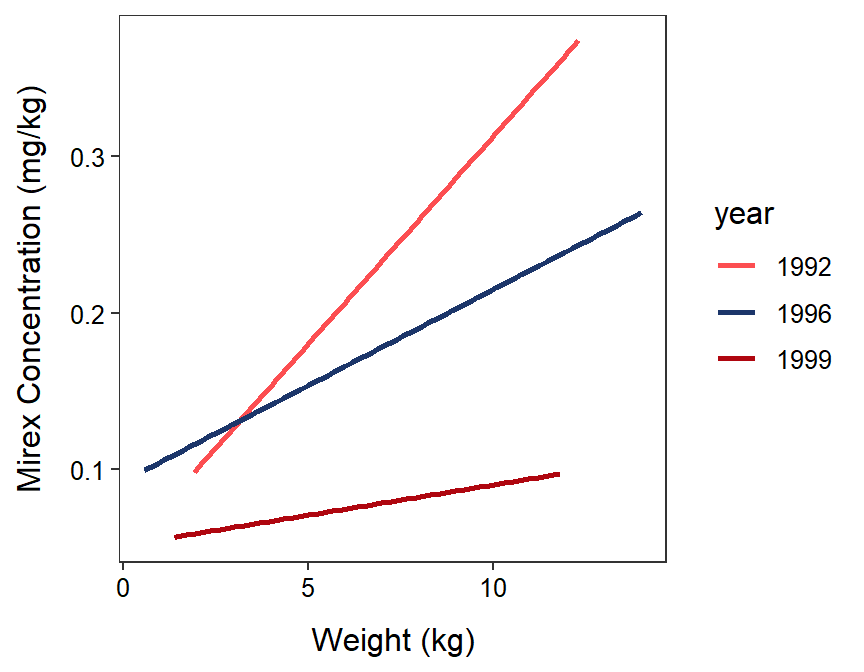
Figure 22.6: Fitted regression lines for mirex in tissue by salmon weight for 1992, 1996, and 1999. Note that the IVR indicated that these lines are not parallel.
If there are more than two groups, then a significant parallel lines test means that at least one group has a different slope. A multiple comparison method (Module 23) is needed to identify which groups have different slopes.
22.7 More Groups (Same Slopes)
For the purposes of having another simple example, suppose that only the first three years from the salmon data are considered.
MirexFirst3 <- filter(Mirex,year %in% c(1977,1982,1986))
ivrY2 <- lm(mirex~weight+year+weight:year,data=MirexFirst3)
anova(ivrY2)
#R> Analysis of Variance Table
#R>
#R> Response: mirex
#R> Df Sum Sq Mean Sq F value Pr(>F)
#R> weight 1 0.32844 0.32844 89.9408 6.064e-14
#R> year 2 0.05719 0.02859 7.8306 0.0008881
#R> weight:year 2 0.00089 0.00044 0.1218 0.8855178
#R> Residuals 66 0.24101 0.00365With these results it is seen that the lines for the three years are parallel (p=0.8855); thus, the relationship between mirex concentration in the tissue and weight of the salmon does not differ among these three years (Figure 22.7). There does appear to be a significant relationship between mirex concentration in the tissue and weight of the salmon (p<0.00005). Finally, it appears that mean mirex concentration in salmon of the same weight differs between at least one pair of years (p=0.0009). Again, in the next module, multiple comparison methods for distinguishing which pairs of groups have different intercepts will be introduced.
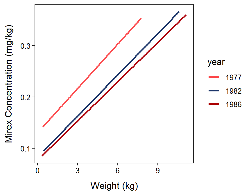
Figure 22.7: Fitted regression lines for mirex in tissue by salmon weight for only 1977, 1982, and 1986. Note that the IVR indicated that these lines are parallel, there is a signficant relationship, and at least one of the lines has a different intercept.
If there are more than two groups, then a significant coincident lines test means that at least one group has a different intercept. A multiple comparison method (Module 23) is needed to identify which groups have different intercepts.