Module 4 Model Comparison

4.1 Competing Models

4.1.1 General

Many hypothesis tests can be cast in a framework of competing models. In this module we will cast the familiar 2-sample t-test in this framework which will then serve as a conceptual foundation for all other models in this course.

The two competing models are generically called the simple and full models (Table 4.1). The simple model is simpler than the full model in the sense that it has fewer parameters. However, the simple model fits the data “worse” than the full model. Thus, determining which model to use becomes a question of balancing “fit” (full model fits better than the simple model) with complexity (full model is more complex than the simple model). Because the simple model corresponds to H₀ and the full model corresponds to H_A, deciding which model to use is the same as deciding which hypothesis is supported by the data.

 

Table 4.1: Differences between the two generic model types.

Model	Parameters	Residual df	Relative Fit	Residual SS	Hypothesis
Simple	Fewer	More	Worse	Larger	Null
Full	More	Less	Better	Smaller	Alternative

 

4.1.2 2-Sample t-Test

Recall that H₀ in a two-sample t-test is that the two population means do not differ (i.e., they are equal). In this hypothesis, if the two means do not differ than a single mean would adequately represent both groups. The general model from Section 3.1⁶ could be specified for this situation as

\[ Y_{ij} = \mu + \epsilon_{ij} \]

where \(Y_{ij}\) is the \(j\)th observation of the response variable in the \(i\)th group, \(\mu\) is the population grand mean, and \(\epsilon_{ij}\) is the “error” for the \(j\)th observation in the \(i\)th group. This model means that μ is the predicted response value for each observation and the model looks like the red line in Figure 4.1.

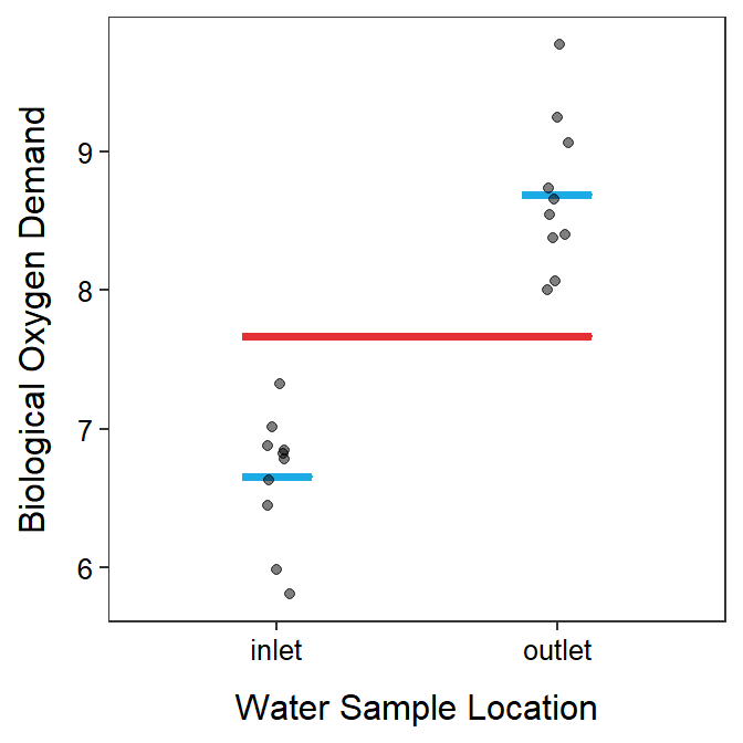
Figure 4.1: Biological oxygen demand versus sample location with group means shown as blue horizontal segments and the grand mean shown as a red horizontal segment.

 

In contrast, H_A in the 2-sample t-test is that the two population means differ (i.e., they are not equal). This hypothesis suggests that two separate means are needed to predict observations in the separate groups. The model for this situation is

\[ Y_{ij} = \mu_{i} + \epsilon_{ij} \]

where \(\mu_{i}\) is the population mean for the \(i\)th group. This model means that \(\mu_{1}\) is the predicted response value for observations in the first group and \(\mu_{2}\) is the predicted response value for observations in the second group. This model looks like the two blue lines in Figure 4.1.

Thus, for a 2-sample t-test, the simple model corresponds to H₀: \(\mu_{1}=\mu_{2}\) (=\(\mu\)), has fewer parameters (i.e., requires only one mean; the red line in the plots above), and fits “worse.”⁷ In contrast, the full model corresponds to H_A: \(\mu_{1}\ne\mu_{2}\), has more parameters (i.e., requires two means; the blue lines in the plots above), and fits “better.”

In the ensuing sections we develop a method to determine if the improvement in “fit” is worth the increase in “complexity.”

 

4.2 Measuring Increase in Fit

4.2.1 SS_Total and SS_Within

Using the residual sum-of-squares (RSS) to measure the lack-of-fit of a model was introduced in Section 3.2.2. Here we apply that concept to measure the lack-of-fit of the simple and full models, which we will then use to see how much “better” the full model fits than the simple model.

The RSS for the simple model using just the grand mean is called SS_Total and is computed with

\[ \text{SS}_{\text{Total}} = \sum_{i=1}^{I}\sum_{j=1}^{n_{i}}\left(Y_{ij}-\bar{Y}_{\cdot\cdot}\right)^{2} \]

where \(I\) is the number of groups (=2 in a 2-sample t-test), \(n_{i}\) is the sample size in the \(i\)th group, and \(\bar{Y}_{\cdot\cdot}\) is the sample grand mean as computed with

\[ \bar{Y}_{\cdot\cdot}= \frac{\sum_{i=1}^{I}\sum_{j=1}^{n_{i}}Y_{ij}}{n} \]

where \(n\) is the sample size across all groups. The \(\bar{Y}_{\cdot\cdot}\) is used here because it is an estimate of the population grand mean, \(\mu\), which is used to make predictions in this simple model.

The formula for SS_Total may look daunting but it is just the sum of the squared residuals computed from each observation relative to the grand mean (Figure 4.2).

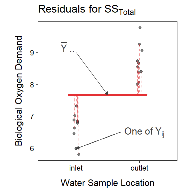
Figure 4.2: Biological oxygen demand versus sample location with the grand mean shown as a red horizontal segment. Residuals from the grand mean are shown by red vertical dashed lines. The sum of these residuals is SS_Total.

 

The RSS for the full model using separate group means is called SS_Within and is computed with

\[ \text{SS}_{\text{Within}} = \sum_{i=1}^{I}\sum_{j=1}^{n_{i}}\left(Y_{ij}-\bar{Y}_{i\cdot}\right)^{2} \]

where \(\bar{Y}_{i\cdot}\) are the sample group means as computed with

\[ \bar{Y}_{\cdot\cdot} = \frac{\sum_{j=1}^{n_{i}}Y_{ij}}{n_{i}} \]

The \(\bar{Y}_{i\cdot}\) are used here because they are an estimate of the population group means, \(\mu_{i}\), which are used to make predictions in this full model. Again, the formula for SS_Within may look imposing but it is just the sum of the squared residuals computed from each observation to the observation’s group mean (Figure 4.3).

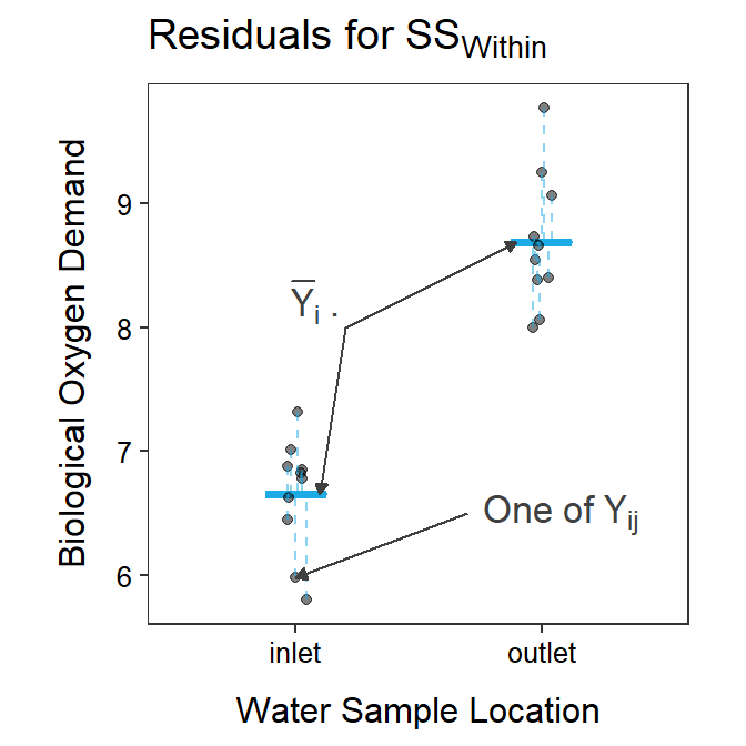
Figure 4.3: Biological oxygen demand versus sample location with the group means shown as blue horizontal segments. Residuals from the group means are shown by blue vertical dashed lines. The sum of these residuals is SS_Within.

 

Thus, SS_Total measures the lack-of-fit of the grand mean to the data or the lack-of-fit of the simple model. SS_Within, in contrast, measures the lack-of-fit of the group means to the data or the lack-of-fit of the full model.

In this example, SS_Total=25.28 and SS_Within=4.60. Because SS_Within is less than SS_Total that means that the full model that uses \(\mu_{i}\) fits the data better than the simple model that uses just \(\mu\).

However, we knew that this was going to happen as the full model always fits better. What we need now is a measure of how much better the full model fits or, equivalently, a measure of how much the lack-of-fit was reduced by using the full model rather than the simple model.

SS_Total measures the lack-of-fit of the simple model, whereas SS_Within measures the lack-of-fit of the full model.

The full model always fits better than the simple model, even if by just a small amount.

4.2.2 SS_Among

A useful property of SS_Total is that it “partitions” into two parts according to the following simple formula

\[ \text{SS}_{\text{Total}} = \text{SS}_{\text{Within}} + \text{SS}_{\text{Among}} \]

A quick re-arrangement of the partitioning of SS_Total shows that

\[ \text{SS}_{\text{Among}} = \text{SS}_{\text{Total}} - \text{SS}_{\text{Within}} \]

Thus, SS_Among records how much the lack-of-fit was reduced by using the full model rather than the simple model. In other words, SS_Among records how much “better” the full model fits the data than the simple model. In our example, SS_Among=25.28-4.60=20.68. Thus, the residual SS from the simple model was reduced by 20.68 when the full model was used.

SS_Among can also be thought of in a different way. It can be algebraically shown that

\[ \text{SS}_{\text{Among}} = \sum_{i=1}^{I}n_{i}\left(\bar{Y}_{i\cdot}-\bar{Y}_{\cdot\cdot}\right)^{2} \]

Again, this looks complicated, but the main part to focus on is \(\bar{Y}_{i\cdot}-\bar{Y}_{\cdot\cdot}\), which shows that SS_Among is primarily concerned with measuring the distance between the group means (i.e., \(\bar{Y}_{i\cdot}\)) and the grand mean (i.e., \(\bar{Y}_{\cdot\cdot}\); Figure 4.4).

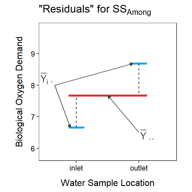
Figure 4.4: Mean biological oxygen demand versus sample location with the grand mean shown as a red horizontal segment and the group means shown as blue horizontal segments. Residuals between the group means and the grand mean are shown by black vertical dashed lines. The sum of these residuals scaled by the group sample sizes is SS_Among.

 

From the figure above, it is seen that SS_Among will increase as the group means become more different. This can also be seen by increasing or decreasing the difference between the group means and the grand mean in the interactive graphic below. [Note how SS_Among (and SS_Total) change.]

 

So, SS_Among is immensely useful – it is a measure of “benefit” that will be used in a “benefit-to-cost” ratio that will ultimately be the “signal” that will be used in a “signal-to-noise” ratio. These ratios are introduced in Sections 4.4 and 4.5. However, next we discuss how to measure the “cost” of using the more complex full model.

SS_Among is the benefit (i.e., reduction in lack-of-fit) from using the full model and will ultimately be used to measure the signal (i.e., relative difference in group means) in the data.

4.3 Measuring Increase in Complexity

In this example, df_Total=20-1 because there is one parameter (the grand mean) in the simple model, and df_Within=20-2 because there are two parameters (the group means) in the full model. The full model uses more parameters and, thus, the residual degrees-of-freedom is reduced – there is a “cost” to using the full model over the simple model. We need a measure of this “cost.”⁸

Interestingly df_Total partitions in the same way as SS_Total; i.e.,

\[ \text{df}_{\text{Total}} = \text{df}_{\text{Within}} + \text{df}_{\text{Among}} \]

A quick re-arrangement of the partitioning of df_Total shows that

\[ \text{df}_{\text{Among}} = \text{df}_{\text{Total}} - \text{df}_{\text{Within}} \]

In this case, df_Among=19-18=1.

Thus, df_Among is the degrees-of-freedom that were “lost” or “used” when the more complex full model was used compared to the less complex simple model. The df_Among is also the difference in number of parameters between the full and simple models. In other words, df_Among is how much more complex (in terms of number of parameters) the full model is compared to the simple model. Thus, df_Among measures the cost of using the full model rather than the simple model.

df_Among is the extra cost (i.e., loss of df due to more parameters to estimate) from using the full rather than simple model.

4.4 “Noise” Variances

MS_Total and MS_Within are measures of the variance⁹ of individuals around the grand mean and group means, respectively. Thus, MS_Total measures the variance or “noise” around the simple model, whereas MS_Within measures the variance or “noise” around the full model.

MS_Total and MS_Within measure “noise” – i.e., variability of observations around a model.

Note that

\[ \text{MS}_{\text{Total}} = \frac{\text{SS}_{\text{Total}}}{\text{df}_{\text{Total}}} = \frac{\sum_{i=1}^{I}\sum_{j=1}^{n_{i}}\left(Y_{ij}-\bar{Y}_{\cdot\cdot}\right)^{2}}{n-1} \]

The double summation simply means to “sum across all individuals.” With this it should be seen that this is same as the variance (\(s^{2}\)) from your introductory statistics course. In other words MS_Total is just the variability of the individuals around a mean that ignores that there are groups.

MS_Total=\(s^{2}\)

Similarly,

\[ \text{MS}_{\text{Within}} = \frac{\text{SS}_{\text{Within}}}{\text{df}_{\text{Within}}} = \frac{\sum_{i=1}^{I}\sum_{j=1}^{n_{i}}\left(Y_{ij}-\bar{Y}_{i\cdot}\right)^{2}}{\sum_{i=1}^{I}n_{i}-I} \]

It is not hard to show algebraically (and for just two groups) that the numerator (top part) is \(n_{1}s_{1}^{2}+n_{2}s_{2}^{2}\) and the denominator (bottom part) is \(n_{1}+n_{2}-2\). With this numerator and denominator, it is evident that MS_Within (for two groups) is the same as the pooled sample variance (\(s_{p}^{2}\)) from the 2-sample t-test.

MS_Within=\(s_{p}^{2}\) from the 2-sample t-test.

4.5 “Signal” Variance (Benefit-to-Cost)

Of course SS_Among divided by df_Among will be MS_Among. However, while MS_Among is still a variance, it has a very different interpretation.

MS_Among is NOT a variance of individuals, rather it is a variance of sample means. Sample means can vary (i.e., not be equal) for two reasons – random sampling variability¹⁰ or the population means are really different.¹¹ In other words, MS_Among – the variance among means – is a combination of “noise” and “signal.” Our goal (next) is to disentangle these two reasons for why the sample means differ to determine if there is a real “signal” or not.

Additionally, MS_Among is a ratio of the “benefit” (i.e., SS_Among) to the “cost” (i.e., df_Among) of using the full model over the simple model. So MS_Among scales the benefit to the cost of using the full model.

 

4.6 Ratio of Variances (Signal-to-Noise)

From the above discussion we have a measure of potential “signal” in MS_Among, but it is contaminated with some “noise.” Additionally, we have a measure of just “noise” around the full model (the model representing the “signal”) in MS_Within. A ratio of this “signal” to “noise” is called an F test statistic; i.e.,

 

\[ \text{F}=\frac{\text{MS}_{\text{Among}}}{\text{MS}_{\text{Within}}} = \frac{\text{Signal}}{\text{Noise}} = \frac{\text{Variance Explained by Full Model}}{\text{Variance Unexplained by Full Model}} \]

 

If the F-ratio is “large,” then “signal” is stronger than the “noise.” A large F-ratio also means that more variability was explained than was unexplained by the full model. Thus, large F-ratio values mean that the full model fits the data significantly better than the simple model, even considering the increased complexity of the full model.

The question now becomes “when is the F-ratio considered large enough to reject the simple model and conclude that the full model is significantly better?” This question is answered by comparing the F-ratio test statistic to an F-distribution.

An F-distribution¹² is right-skewed, with the exact shape of the distribution dictated by two separate df – called the numerator and denominator df, respectively. The numerator df is equal to the df used in MS_Among, whereas the denominator df is equal to the df used in MS_Within. The p-value is always computed as the area under the F-distribution curve to the right of the observed F-ratio test statistic (Figure 4.5).¹³

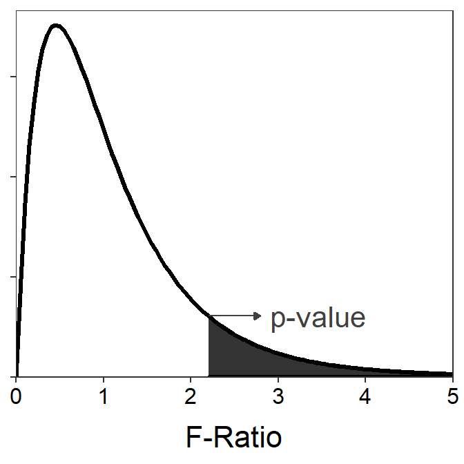
Figure 4.5: An F distribution with 4 numerator and 20 denominator degrees-of-freedom. The shaded area demonstrates calculating a p-value for an F-ratio of 2.2.

 

From all of the previous discussion, it can be seen that …

• a small p-value comes from a large F-ratio, which comes from
• a large MS_Among relative to MS_Within, which means that
• the full model explains more variability than is left unexplained and that the “signal” is much greater than the “noise,” which means that
• the full model does fit significantly better than the simple model (even given the increased complexity), and, thus,
• the means are indeed different.

This cascade of measures can be explored with the dynamic graphic below.

A small p-value results in concluding that the group means are significantly different.

4.7 ANOVA Table

The degrees-of-freedom (df), sum-of-squares (SS), mean-squares (MS), F-ratio test statistic (F), and corresponding p-value are summarized in an analysis of variance (ANOVA) table.¹⁴ The ANOVA table contains rows that correspond to the different measures discussed above: among,¹⁵ within,¹⁶ and total. The df and SS are shown for each source, but the MS is shown only for the within and among sources because MS_Among+MS_Within ≠ MS_Total.

An ANOVA table for the BOD measurements at the inlet and outlet sources to the aquaculture facility is in Table 4.2. Note that R does not show the total row that most softwares do.

Table 4.2: An ANOVA table for biological oxygen demand measurements at two locations of the aquaculture facility. Note that the “Total” row is not shown.

	Df	Sum Sq	Mean Sq	F value	Pr(>F)
src	1	20.6756	20.6756	80.8912	0
Residuals	18	4.6008	0.2556

 

These results indicate that H₀ should be rejected (i.e., F-test p-value <0.00005). Thus, the full model fits the data significantly better than the simple model even given the increased complexity and sampling variability. Therefore, there is a significant difference in mean BOD between the two source locations.

In addition to the primary objective of comparing the full and simple models and making a conclusion about the equality of group means, several other items of interest can be identified from an ANOVA table. Using the table above as an example, note that

• the variance within groups is 0.2556 (=MS_Within=MS_{Residuals=\(s_{p}^{2}\)), and}
• the common variance about the mean is 1.3303 (=MS_Total=\(s^{2}\)=\(\frac{20.6756+4.6008}{1+18}\)).

SS and df partition, but MS do not! Do not add MS_Among and MS_Within to get MS_Total, instead divide SS_Total by df_Total.

 

4.8 Two-Sample t-Test Revisited: Using Linear Models

The models for a two-sample t-test can be fit and assessed with lm(). This function requires the same type of formula for its first argument – response~groups – and a data.frame in the data= argument as described for t.test() in Section 2.2. The results of lm() should be assigned to an object so that specific results can be selectively extracted from it. For example, the ANOVA table results are extracted with anova(). In addition, coefficient results¹⁷ can be extracted with coef() and confint(), noting that I like to “column-bind” the coefficients and confidence intervals together for a more succinct representation.

aqua.lm <- lm(BOD~src,data=aqua)
anova(aqua.lm)

#R>  Analysis of Variance Table
#R>  
#R>  Response: BOD
#R>            Df  Sum Sq Mean Sq F value    Pr(>F)
#R>  src        1 20.6756 20.6756  80.891 4.449e-08
#R>  Residuals 18  4.6008  0.2556

cbind(ests=coef(aqua.lm),confint(aqua.lm))

#R>                ests    2.5 %   97.5 %
#R>  (Intercept) 6.6538 6.317917 6.989683
#R>  srcoutlet   2.0335 1.558489 2.508511

From these results, note:

• The p-value in the ANOVA table is the same as that computed from t.test().
• The coefficient for srcoutlet is the same as the difference in the group means computed with t.test().
• The F test statistics in the ANOVA table equals the square of the t test statistic from t.test(). This is because an F with 1 numerator and v denominator df exactly equals the square of a t with v df.

Thus, the exact same results for a two-sample t-test are obtained whether the analysis is completed in the “traditional” manner (i.e., with t.test()) or with competing models (i.e., using lm()). This concept will be extended in subsequent modules.

 

4.9 One More Look at MS and F-test

Recall from your introductory statistics course that a sampling distribution is the distribution of a statistic from all possible samples. For example, the Central Limit Theorem states that the distribution of sample means is approximately normal, centered on μ, with a standard error of \(\frac{\sigma}{\sqrt{n}}\) as long as assumptions about the sample size are met. Further recall that the sampling distribution of the sample means is centered on μ because the sample mean is an unbiased estimator of μ. Similarly, it is also known that the center of the sampling distribution of \(s^{2}\) is equal to \(\sigma^{2}\) because \(s^{2}\) is an unbiased estimate of \(\sigma^{2}\).

MS_Within and MS_Among are statistics just as \(\bar{x}\) and \(s^{2}\) are statistics. Thus, MS_Within and MS_Among are subject to sampling variability and have sampling distributions. It can be shown¹⁸ that the center of the sampling distribution of MS_Within is \(\sigma_{p}^{2}\) and the center of the sampling distribution of MS_Among is

\[ \sigma_{p}^{2} + \frac{\sum_{i=1}^{I}n_{i}\left(\mu_{i}-\mu\right)^{2}}{I-1} \]

Thus, MS_Among consists of two “sources” of variability. The first source (\(\sigma_{p}^{2}\)) is the natural variability that exists among individuals (around the group means). The second source \(\left(\frac{\sum_{i=1}^{I}n_{i}\left(\mu_{i}-\mu\right)^{2}}{I-1}\right)\) is related to differences among the group means. Therefore, if the group means are all equal – i.e., \(\mu_{1}\)=\(\mu_{2}\)= \(\cdots\) = \(\mu_{I}\) = \(\mu\) – then the second source of variability is equal to zero and MS_Among will equal MS_Within. As soon as the groups begin to differ, the second source of variability will be greater than 0 and MS_Among will be greater than MS_Within.

From this, it follows that if the null hypothesis of equal population means is true (i.e., one mean fits all groups), then the center of the sampling distribution of both MS_Within and MS_Among is \(\sigma_{p}^{2}\). Therefore, if the null hypothesis is true, then the F test-statistic is expected to equal 1, on average, which will always result in a large p-value and a DNR H₀ conclusion. However, if the null hypothesis is false (i.e., separate means are needed for all groups), then the center of the sampling distribution of MS_Within is \(\sigma_{p}^{2}\) but the center of the sampling distribution of MS_Among is \(\sigma_{p}^{2}\) + “something,” where the “something” is greater than 0 and gets larger as the means become “more different.” Thus, if the null hypothesis is false then the F test-statistic is expected to be greater than 1 and will get larger as the null hypothesis gets “more false.” This analysis of sampling distribution theory illustrates once again that (1) MS_Among consists of multiple sources of variability and (2) “large” values of the F test-statistic indicate that the null hypothesis is incorrect.

 

---

6. Generally, Observation = Model Prediction + Error↩︎

7. We will be more objective in the following sections, but an examination of the plot above clearly shows that the red line does not represent the observations well.↩︎

8. The “cost” is obviously 1 in this simple case.↩︎

9. As discussed in Section 3.4, SS are not true variances until they are divided by their df and become mean-squares (MS).↩︎

10. That is sample means will vary from sample to sample even if the population means are not different.↩︎

11. If the population means are different then one would expect the means from samples of those populations to also be different.↩︎

12. An F-distribution occurs whenever the ratio of two variances is calculated.↩︎

13. If the F-ratio is computed by hand, then distrib() with distrib="f", df1=, df2=, and lower.tail=FALSE may be used to calculate the corresponding p-value.↩︎

14. An ANOVA table does not necessarily mean that an “analysis of variance” method was used. It turns out that all general linear models are summarized with an ANOVA table, regardless of whether a one- or two-way ANOVA method was used.↩︎

15. Labeled as the factor variable in most statistical software packages including R – that variable was called src in this example.↩︎

16. Labeled as residuals in R and error in other statistical software packages.↩︎

17. The coefficient results will be discussed in more detail in Module 5.↩︎

18. This derivation is beyond the scope of this course.↩︎