Module 14 Hypothesis Testing - Errors
In Module 13 we examined the concept of hypothesis testing and showed how a p-value is calculated and used to reject or not reject H0. The basic concept there is that if the p-value is small (<α) then it unlikely that the observed statistic would come from a population with the parameter in the H0. It is important to note the word unlikely in this statement. It is possible that the observed statistic would come from this population, just unlikely. In the case where this unlikely event actually happened, we would make an error in our conclusion about H0. These errors are discussed in this module.
14.1 Error Types
The goal of hypothesis testing is to make a decision about H0. Unfortunately, because of sampling variability, there is always a risk of making an incorrect decision. Two types of incorrect decisions can be made (Table 14.1). A Type I error occurs when a true H0 is falsely rejected. In other words, even if H0 is true, there is a chance that a rare sample will occur and H0 will be deemed incorrect. A Type II error occurs when a false H0 is not rejected.
| Truth about Popn | Decision from Test | Error Type |
|---|---|---|
| H0 is true | Reject H0 | Type I (\(\alpha\)) |
| H0 is true | DNR H0 | – |
| HA is true | Reject H0 | – |
| HA is true | DNR H0 | Type II (\(\beta\)) |
It is important to be able to articulate what Type I and a Type II errors are within the context of a specific situation. For example, suppose that if the mean abundance of a rare plant in a particular area drops below 0.5 plants per m2 then there is a real concern that that plant will become extinct. A researcher may conduct a study to determine if the mean abundance of this plant has dropped below the 0.5 m2 threshold or not. The null and alternative hypotheses would be
- H0: μ=0.5, where μ is the mean abundance of the plant per m2
- HA: μ<0.5
Before articulating what the errors would be in this example, it is useful to write in words what the hypotheses are within the context of the situation.
- H0: “abundance at or above the threshold; population not at risk of extinction”
- HA: “abundance below the threshold; population at risk of extinction”
From the definition of a Type I error (i.e., incorrectly rejecting a true H0), a Type I error occurs if we conclude that HA is true when H0 is really true. In this scenario then, a Type I error would be concluding that the abundance of the plant is low (think HA is true) when the abundance is really not low (H0 is really true) or concluding that the population is at risk of extinction when the population is really not at risk of extinction.
From the definition of a Type II error (i.e., incorrectly not rejecting a false H0), a Type II error is concluding that H0 is true when HA is really true. In this scenario then, a Type II error is concluding that the abundance of the plant is not low (think H0 is true) when the abundance is really low (HA is really true) or concluding that the population is not at risk of extinction when the population is really at risk of extinction.
14.2 Error Rates
The decision in the Square Lake example of Module 13 was a Type II error because H0:μ=105 was not rejected even though we know that μ=98.06 (Table 2.1). Unfortunately, in real life, it will never be known exactly when a Type I or a Type II error has been made because the true μ is not known. However, the rates at which these errors are made can be considered.
The probability of making a Type I error is set when α is chosen. Thus, the researcher can largely choose the rate at which they will make a Type I error. The probability of a Type II error is denoted by β, which is never known because calculating β requires knowing the true but unknown μ. Decisions can be made, however, that affect the magnitude of β (Figure 14.1).
There are two items that affect β that a researcher can control – the size of α and n. The β decreases as α increases (Figure 14.1); i.e., the researcher is reducing Type II errors by allowing for more Type errors. In other words, the researcher is simply “trading errors,” which may be appropriate if a Type II error is more egregious than a Type I error. The β also decreases with increasing n (Figure 14.1); i.e., fewer errors are made as more information is gathered. Of these two choices, reducing β by increasing n is generally more beneficial because it does not result in an increase in Type I errors as would occur with increasing α.
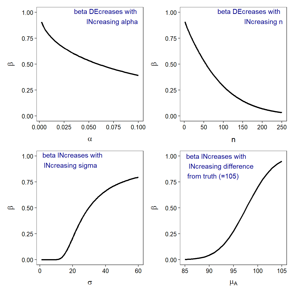
Figure 14.1: The relationship between one-tailed (lower) β and α, n, actual mean (μA), and σ. In all situations where the variable does not vary, μ0=105, μA=98.06, σ=31.49, n=50, and α=0.05.
The value of β is als related to two items that a researcher cannot control. The β increases as the difference between the hypothesized mean (μ0) and the actual mean (μA) decreases (Figure 14.1). This means that more Type II errors will be made when the hypothesized and actual mean are close together. In other words, more Type II errors are made when it is harder to distinguish the hypothesized mean from the actual mean.
In addition, β increases with increasing amounts of natural variability (i.e., σ; Figure 14.1). In other words, more Type II errors are made when there is more variability among individuals.
A researcher cannot control the difference between μ0 and μA or the value of σ. However, it is important to know that if a situation with a “large” amount of variability is encountered or the difference to be detected is small, the researcher will need to increase n to reduce β. For example, if n could be doubled in the Square Lake example to 100, then β (for H0:μ=105) would decrease to approximately 0.18 (Figure 14.1).
Statistical Power
A concept that is very closely related to decision-making errors is the idea of statistical power, or just power for short. Power is the probability of correctly rejecting a false H0. In other words, it is the probability of detecting a difference from the hypothesized value if a difference really exists. Power is used to demonstrate how sensitive a hypothesis test is for identifying a difference. High power related to a H0 that is not rejected implies that the H0 really should not have been rejected. Conversely, low power related to a H0 that was not rejected implies that the test was very unlikely to detect a difference, so not rejecting H0 is not surprising nor particularly conclusive. Power is equal to 1-β.
14.3 Test Statistics and Effect Sizes
Instead of reporting the observed statistic and the resulting p-value, it may be of interest to know how “far” the observed statistic was from the hypothesized value of the parameter. This is easily calculated with
\[ \text{Observed Statistic}-\text{Hypothesized Parameter} \]
where “Hypothesized Parameter” represents the specific value in H0. However, the meaning of this difference is difficult to interpret without an understanding of the standard error of the statistic. For example, a difference of 10 between the observed statistic and the hypothesized parameter seems “very different” if the standard error is 3 but does not seem “different” if the standard error is 15 (Figure 14.2).
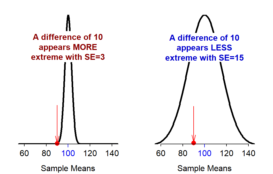
Figure 14.2: Sampling distribution of samples means with SE=3 (Left) and SE=15 (Right). A single observed sample mean of 90 (a difference of 10 from the hypothesized mean of 100) is shown by the red dot and arrow.
The difference between the observed statistic and the hypothesized parameter is standardized to a common scale by dividing by the standard error of the statistic. The result is called a test statistic and is generalized with
\[ \text{Test Statistic} = \frac{\text{Observed Statistic}-\text{Hypothesized Parameter}}{\text{SE}_{\text{Statistic}}} \]
Thus, the test statistic measures how many standard errors the observed statistic is away from the hypothesized parameter.60 A relatively large value of the test statistic is indicative of a difference that is likely not due to randomness (i.e., sampling variability) and suggests that the null hypothesis should be rejected.
The test statistic in the Square Lake Example is \(\frac{100-105}{\frac{31.49}{\sqrt{50}}}\)=-1.12. Thus, the observed mean total length of 100 mm is 1.12 standard errors below the null hypothesized mean of 105 mm. From our experience, a little over one SE from the mean is not “extreme” and, thus, it is not surprising that the null hypothesis was not rejected.
There are other forms for calculating test statistics, but all test statistics retain the general idea of scaling the difference between what was observed and what was expected from the null hypothesis in terms of sampling variability. Even though there is a one-to-one relationship between a test statistic and a p-value, a test statistic is often reported with a hypothesis test to give another feel for the magnitude of the difference between what was observed and what was predicted.