Module 3 Read External Data Files
Most realistic data has more than a few individuals and is, thus, not easily entered using data.frame() or tibble() as shown in Section 2.3. Rather these data are often entered and stored in a spreadsheet or database that is external to R and must then be read into R. This module describes how data should be entered into a spreadsheet and then how that data is read into R.
3.1 Entering Data
Tidy data (see Section 2.4) is often entered into a spreadsheet program such as Microsoft Excel or Google Sheets. The spreadsheet should be organized with variables in columns and individuals in rows, with the exception that the first row should contain variable names. The example spreadsheet below shows the length (cm), weight (kg), and capture location data for a small sample of Black Bears.
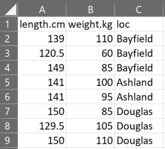
Variable names should NOT contain spaces. For example, don’t use “total length” or “length (cm).” If you feel the need to have longer variable names, then separate the parts with a period (e.g., “length.cm”) or an underscore (e.g., “length_cm”). Variable names can NOT start with numbers or contain “special” characters such as “~,” “!” “&,” “@,” etc. Furthermore, numerical measurements should NOT include units (e.g., don’t use “7 cm”). Finally, for categorical data, make sure that all categories are consistent (e.g., do not use both “bayfield” and “Bayfield”).
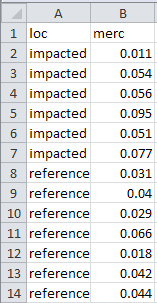
When entering data make sure to follow the three rules of tidy data (see Section 2.4). For example, the following data are methyl mercury levels recorded in mussels captured from “impacted” and “reference” locations.
  impacted   0.011  0.054  0.056  0.095  0.051  0.077
  reference  0.031  0.040  0.029  0.066  0.018  0.042  0.044
As described in Section 2.4, one “observation” (i.e., row) is a methyl mercury measurement on a mussel AND which group the mussel belongs. The rules for tidy data dictate two columns (one for each of the two variables recorded) and 13 rows (one for each observation of a mussel). Thus, these data would be entered into the spreadsheet as below.
3.2 Saving the External File
The spreadsheet may be saved in the format of the spreadsheet program (e.g., as an Excel file) to be read into R.
It is also common to save the file as a comma separated values (CSV) file to be read into R. The advantage of a CSV file is that these files are small and, because they do not require any special software (e.g., Excel) to read, they are very likely to always be able to be read into R. The next two sections describe how to create CSV files in Excel and GoogleSheets.
3.2.1 Excel
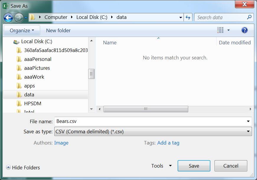
An Excel worksheet is saved as a CSV file by selecting the File menu and Save As submenu, which will produce the dialog box below. In this dialog box, change “Save as type” to “CSV (Comma delimited),”9, provide a file name (do not put any periods in the name), select a location to save the file (this should be in your RStudio project folder), and press “Save.” Two “warning” dialog boxes may then appear – select “OK” for the first and “YES” for the second. You can now close the spreadsheet file.10
3.2.2 Google Sheets
A Google Sheet can be made available as a CSV file by selecting the File menu, Share submenu, and Publish to web submenu. In the ensuing dialog box, change “Entire Document” to the name of the sheet you want to publish and “Web Page” to “Comma-separated values (.csv)” under the “Link” tab.
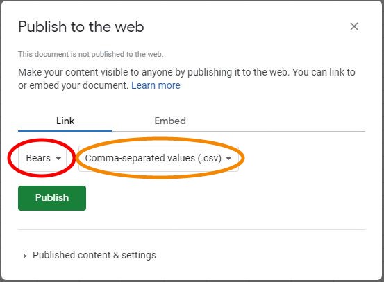
Then press the “Publish” button and press OK when asked to confirm publishing.
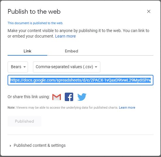
Finally, select and copy (CTRL-C or CMD-C) the entire link shown in the box above. This link will be used as described in the next section.
3.3 Reading an External File
3.3.1 CSV Files
CSV files may be read into R with read.csv() from base R or read_csv() from tidyverse. For most of our applications there will be little functional difference between these two functions. However, read_csv() is faster than read.csv() and can be a little “smarter” about the way it imports certain columns.11 In addition, it is a bit more transparent about what it is doing. For those reasons, read_csv() will be used in this course.
An object saved from read_csv() will be a tibble.
The first argument to read_csv() is the filename, which may include a partial path relative to your working directory, a full path to the file, or be a valid URL. For example, the code below reads “Bears.csv” from the “data” folder in my working directory12 and stores the result in the bears object. Here, I used file.path() to combine the folder names in the partial path with the filename because file.path() creates a path that will be correct for your operating system.13
bears <- read_csv(file.path("data","Bears.csv"))
bears
#R> # A tibble: 8 x 3
#R> length.cm weight.kg loc
#R> <dbl> <dbl> <chr>
#R> 1 139 110 Bayfield
#R> 2 120. 60 Bayfield
#R> 3 149 85 Bayfield
#R> 4 141 100 Ashland
#R> 5 141 95 Ashland
#R> 6 150 85 Douglas
#R> 7 130. 105 Douglas
#R> 8 150 110 DouglasThe filename argument could also be the link to the published Google Sheet (from above).
bears <- read_csv("https://docs.google.com/spreadsheets/d/e/2PACX-1vQaxD9tvwL29MydISlYw4bVXrw6-rvkEbT_2qFGxw7HuYX6M3h83aIYT4eZ-mrrEfJf8y5Q8p1Rkn4Z/pub?gid=522647677&single=true&output=csv")
bears
#R> # A tibble: 8 x 3
#R> length.cm weight.kg loc
#R> <dbl> <dbl> <chr>
#R> 1 139 110 Bayfield
#R> 2 120. 60 Bayfield
#R> 3 149 85 Bayfield
#R> 4 141 100 Ashland
#R> 5 141 95 Ashland
#R> 6 150 85 Douglas
#R> 7 130. 105 Douglas
#R> 8 150 110 DouglasThe URL can be any valid URL and does not have to be just from a published Google Sheet. For example, the following code reads a CSV from this page that lists information about every player who has played in the National Basketball Association (NBA).
players <- read_csv("https://sports-statistics.com/database/basketball-data/nba/NBA-playerlist.csv")
players
#R> # A tibble: 4,393 x 15
#R> ...1 DISPLAY_FIRST_LAST DISPLAY_LAST_COMMA_FIRST FROM_YEAR GAMES_PLAYED_FL~
#R> <dbl> <chr> <chr> <dbl> <chr>
#R> 1 0 Alaa Abdelnaby Abdelnaby, Alaa 1990 Y
#R> 2 1 Zaid Abdul-Aziz Abdul-Aziz, Zaid 1968 Y
#R> 3 2 Kareem Abdul-Jabbar Abdul-Jabbar, Kareem 1969 Y
#R> 4 3 Mahmoud Abdul-Rauf Abdul-Rauf, Mahmoud 1990 Y
#R> 5 4 Tariq Abdul-Wahad Abdul-Wahad, Tariq 1997 Y
#R> 6 5 Shareef Abdur-Rahim Abdur-Rahim, Shareef 1996 Y
#R> 7 6 Tom Abernethy Abernethy, Tom 1976 Y
#R> 8 7 Forest Able Able, Forest 1956 Y
#R> 9 8 John Abramovic Abramovic, John 1946 Y
#R> 10 9 Alex Abrines Abrines, Alex 2016 Y
#R> # ... with 4,383 more rows, and 10 more variables:
#R> # OTHERLEAGUE_EXPERIENCE_CH <chr>, PERSON_ID <dbl>, PLAYERCODE <chr>,
#R> # ROSTERSTATUS <dbl>, TEAM_ABBREVIATION <chr>, TEAM_CITY <chr>,
#R> # TEAM_CODE <chr>, TEAM_ID <dbl>, TEAM_NAME <chr>, TO_YEAR <dbl>
The read_csv() function provides a variety of options that will help you correctly load CSV files that may be “quirky” in some respects. Use skip.lines= to skip, for example, the first two lines in a CSV file that do not contain data (perhaps they hold comments).
tmp <- read_csv(file.path("data","Bears_SkipLines.csv"),skip=2)
tmp
#R> # A tibble: 8 x 3
#R> length.cm weight.kg loc
#R> <dbl> <dbl> <chr>
#R> 1 139 110 Bayfield
#R> 2 120. 60 Bayfield
#R> 3 149 85 Bayfield
#R> 4 141 100 Ashland
#R> 5 141 95 Ashland
#R> 6 150 85 Douglas
#R> 7 130. 105 Douglas
#R> 8 150 110 DouglasAlternatively, use comment= to identify leading characters that identify lines in the data file that are comments and should not be read as data.
tmp <- read_csv(file.path("data","Bears_Comment.csv"),comment="#")
tmp
#R> # A tibble: 8 x 3
#R> length.cm weight.kg loc
#R> <dbl> <dbl> <chr>
#R> 1 139 110 Bayfield
#R> 2 120. 60 Bayfield
#R> 3 149 85 Bayfield
#R> 4 141 100 Ashland
#R> 5 141 95 Ashland
#R> 6 150 85 Douglas
#R> 7 130. 105 Douglas
#R> 8 150 110 DouglasOften data may be missing. By default, R treats NA in the data frame as missing data. If all missing data is coded with NA then read_csv() will handle this properly. For example, note the NAs in the second and eighth rows below after reading this data file.
tmp <- read_csv(file.path("data","Bears_Missing1.csv"))
tmp
#R> # A tibble: 8 x 3
#R> length.cm weight.kg loc
#R> <dbl> <dbl> <chr>
#R> 1 139 110 Bayfield
#R> 2 NA 60 Bayfield
#R> 3 149 85 Bayfield
#R> 4 141 100 Ashland
#R> 5 141 95 Ashland
#R> 6 150 85 Douglas
#R> 7 130. 105 Douglas
#R> 8 150 110 <NA>However, some researchers may denote missing data with other codes. For example, the data file read below used “-” to denote missing data. In cases like this, use na= to dictate which codes should be “missing” and converted to NA in the data frame object.
tmp <- read_csv(file.path("data","Bears_Missing2.csv"),na="-")
tmp
#R> # A tibble: 8 x 3
#R> length.cm weight.kg loc
#R> <dbl> <dbl> <chr>
#R> 1 139 110 Bayfield
#R> 2 NA 60 Bayfield
#R> 3 149 85 Bayfield
#R> 4 141 100 Ashland
#R> 5 141 95 Ashland
#R> 6 150 85 Douglas
#R> 7 130. 105 Douglas
#R> 8 150 110 <NA>In other instances, the research may have sloppily used multiple codes for missing data. In these instances (as with this file), set na= to a vector of all codes to be converted to NA in the data frame object.
tmp <- read_csv(file.path("data","Bears_Missing3.csv"),na=c("NA","NAN","-"))
tmp
#R> # A tibble: 8 x 3
#R> length.cm weight.kg loc
#R> <dbl> <dbl> <chr>
#R> 1 139 110 <NA>
#R> 2 NA 60 Bayfield
#R> 3 149 85 Bayfield
#R> 4 141 100 Ashland
#R> 5 NA 95 Ashland
#R> 6 150 85 Douglas
#R> 7 130. 105 Douglas
#R> 8 150 110 <NA>
The examples above will serve you well for most files read in this class, with the possible exception of files that contain variables with dates. Handling dates is discussed in Module 9.
3.3.2 Excel Files
Some researchers prefer to save data entered in Excel as an Excel workbook rather than a CSV file. The main argument here is that saving to a CSV often results in two files – an Excel workbook file and a CSV file. It is generally bad practice to have your data in two files as you may update the Excel file and forget to save it to the CSV file or you may update the CSV file and forget to also update the Excel file. Regardless of the reason, data can generally be read from an Excel file into R.
The read_excel() function from the readxl package provides a coherent process for reading data from an Excel workbook. The first argument to read_excel() is the name of the Excel file, possibly with path information. By default read_excel() reads the first sheet in the Excel workbook. The example below reads the first sheet of the “DataExamples.xlsx” workbook in the “data” folder.14
tmp <- readxl::read_excel(file.path("data","DataExamples.xlsx"))
tmp
#R> # A tibble: 8 x 3
#R> length.cm weight.kg loc
#R> <dbl> <dbl> <chr>
#R> 1 139 110 Bayfield
#R> 2 120. 60 Bayfield
#R> 3 149 85 Bayfield
#R> 4 141 100 Ashland
#R> 5 141 95 Ashland
#R> 6 150 85 Douglas
#R> 7 130. 105 Douglas
#R> 8 150 110 DouglasData on specific sheets can be read by including the sheet name in sheet=. Additionally, lines at the top of the sheet can be skipped with skip= as described for read_csv(). For example, the code below reads the data after the first two lines in the “Bears_SkipLines” worksheet in the same Excel workbook.
tmp <- readxl::read_excel(file.path("data","DataExamples.xlsx"),
                          sheet="Bears_SkipLines",skip=2)
tmp
#R> # A tibble: 8 x 3
#R> length.cm weight.kg loc
#R> <dbl> <dbl> <chr>
#R> 1 139 110 Bayfield
#R> 2 120. 60 Bayfield
#R> 3 149 85 Bayfield
#R> 4 141 100 Ashland
#R> 5 141 95 Ashland
#R> 6 150 85 Douglas
#R> 7 130. 105 Douglas
#R> 8 150 110 DouglasMissing data is handled exactly as described for read_csv().
tmp <- readxl::read_excel(file.path("data","DataExamples.xlsx"),
                          sheet="Bears_Missing3",na=c("NA","NAN","-"))
tmp
#R> # A tibble: 8 x 3
#R> length.cm weight.kg loc
#R> <dbl> <dbl> <chr>
#R> 1 139 110 <NA>
#R> 2 NA 60 Bayfield
#R> 3 149 85 Bayfield
#R> 4 141 100 Ashland
#R> 5 NA 95 Ashland
#R> 6 150 85 Douglas
#R> 7 130. 105 Douglas
#R> 8 150 110 <NA>
In general, read_excel() works best if the data are arranged in a rectangle starting in cell “A1.” However, read_excel() can handle different organizations of data in the worksheet as described here. Researchers may also use multiple header rows in their Excel worksheet; e.g., variables names in the first row, variable units in the second row. This provides a strategy for reading data arranged in such a way.
3.3.3 Google Sheets
It is also possible to read a file directly from Google Sheets using functions in the googlesheets4 package as described here. Using this package to read directly from Google Sheets requires you to authorize R to access your Google Sheets.
3.3.4 Other Formats
Data may be stored in other, less common formats. A few examples of functions to read these other formats are listed below.
read_csv2()(fromtidyverse) for fields separated by semi-colons (rather than commas) as is common in Europe.read_tsv()(fromtidyverse) for fields separated by tabs (rather than commas). An example is in Section 9.7.2.read_fwf()(fromtidyverse) for fields that are a fixed width.read_sav()(fromhaven) for “.sav” files from SPSS.read_sas()(fromhaven) for “.sas7bdat” and “.sas7bcat” files from SAS.read_dta()(fromhaven) for “.dta” files from Stata.
There are several choices for CSV files here; do NOT choose the one with “UTF-8” in the name.↩︎
You may be asked to save changes – you should say “No.”↩︎
How
read_csv()identifies the class of data in a column is described here↩︎If using an RStudio project then the working directory will be the project’s directory.↩︎
Windows and Mac OS handle paths differently; this function avoids that complication.↩︎
I use the
readxl::read_excel()construct here rather than loading thereadxlpackage and then simply usingread_excel()because this is the only function that I will use fromreadxl. Thus, I am not loading unneeded functions into my work environment.↩︎