Introduction
library(FSAdata) # for data
library(FSA)     # for vbFuns(), vbStarts(), confint.bootCase()
library(car)     # for Boot()
library(dplyr)   # for filter(), mutate()
library(ggplot2)
In a previous post I demonstrated how to make a plot that illustrated the fit of a von Bertalanffy growth function (VBGF) to data. In this post, I will demonstrate how to show the VBGF fits for two or more groups (e.g., sexes, locations, years). Here I will again use the lengths and ages of Lake Erie Walleye (Sander vitreus) captured during October-November, 2003-2014. These data are available in my FSAdata package and formed many of the examples in Chapter 12 of the Age and Growth of Fishes: Principles and Techniques book. My primary interest is in the tl (total length in mm), age, and sex variables (see here for more details). I will focus initially on Walleye from location “1” captured in 2014 (as an example).
data(WalleyeErie2)
w14T <- filter(WalleyeErie2,year==2014,loc==1)
The workflow below requires the predict2() and vb() functions that were created in the previous post.
vb <- vbFuns()
predict2 <- function(x) predict(x,data.frame(age=ages))
Fitting all von Bertalanffy Growth Functions
The key to constructing plots with multiple VBGF trajectories is to create a “long format” data.frame of predicted mean lengths-at-age with associated bootstrap confidence intervals. In this format one row corresponds to a single “group” and age with columns (variabls) that identify the “group”, age”, predicted mean length, and the lower and upper values for the confidence interval. There is likely many ways to construct such a data.frame, but a loop over the “groups” (i.e., sexes) is used below
Begin by finding the range of ages for both sexes so that the confidence polygon can be restricted to observed ages.
agesum <- group_by(w14T,sex) %>%
  summarize(minage=min(age),maxage=max(age))
agesum
## # A tibble: 2 x 3
## sex minage maxage
## <fct> <int> <int>
## 1 female 0 11
## 2 male 1 11To simplify coding below, the levels and number of “groups” are saved into objects.
( sexes <- levels(w14T$sex) )## [1] "female" "male"( nsexes <- length(sexes) )## [1] 2In the loop across sexes, the VBGF will be fit for each sex and parameter estimates will be saved into cfs, confidence intervals for the parameter estimates into cis, predicted mean lengths-at-age for all ages considered in preds1, and predicted mean lengths-at-age for only observed ages in preds2. These objects are initialized with NULL prior to starting the loop.1
cfs <- cis <- preds1 <- preds2 <- NULLThe code inside the loop follows the same logic as shown in the previous post for fitting the VBGF to one group.2
for (i in 1:nsexes) {
  ## Loop notification (for peace of mind)
  cat(sexes[i],"Loop\n")
  ## Isolate sex's data
  tmp1 <- filter(w14T,sex==sexes[i])
  ## Fit von B to that sex
  sv1 <- vbStarts(tl~age,data=tmp1)
  fit1 <- nls(tl~vb(age,Linf,K,t0),data=tmp1,start=sv1)
  ## Extract and store parameter estimates and CIs
  cfs <- rbind(cfs,coef(fit1))
  boot1 <- Boot(fit1)
  tmp2 <-  confint(boot1)
  cis <- rbind(cis,c(tmp2["Linf",],tmp2["K",],tmp2["t0",]))
  ## Predict mean lengths-at-age with CIs
  ##   preds1 -> across all ages
  ##   preds2 -> across observed ages only
  ages <- seq(-1,12,0.2)
  boot2 <- Boot(fit1,f=predict2)
  tmp2 <- data.frame(sex=sexes[i],age=ages,
                     predict(fit1,data.frame(age=ages)),
                     confint(boot2))
  preds1 <- rbind(preds1,tmp2)
  tmp2 <- filter(tmp2,age>=agesum$minage[i],age<=agesum$maxage[i])
  preds2 <- rbind(preds2,tmp2)
}
## female Loop
## male LoopThe cfs, cis, preds1, and preds2 objects will have poorly named rows, columns, or both after the loop. These deficiencies are corrected below.
rownames(cfs) <- rownames(cis) <- sexes
colnames(cis) <- paste(rep(c("Linf","K","t0"),each=2),
                       rep(c("LCI","UCI"),times=2),sep=".")
colnames(preds1) <- colnames(preds2) <- c("sex","age","fit","LCI","UCI")
The preds1 and preds2 objects now contain the predicted mean lengths-at-age with associated confidence intervals in the desired long format.
headtail(preds1) # predicted lengths-at-age w/ CIs for ALL ages## sex age fit LCI UCI
## V1 female -1.0 63.17547 12.47969 105.7263
## V2 female -0.8 103.98483 62.48840 138.8930
## V3 female -0.6 141.94750 108.32876 170.5116
## V641 male 11.6 568.09475 552.38131 582.0849
## V651 male 11.8 568.48780 552.59109 582.7325
## V661 male 12.0 568.85535 552.79664 583.5140headtail(preds2) # predicted lengths-at-age w/ CIs for OBSERVED ages## sex age fit LCI UCI
## 1 female 0.0 240.6728 224.6318 254.2693
## 2 female 0.2 269.1007 257.1073 279.3463
## 3 female 0.4 295.5456 286.6625 302.9567
## 105 male 10.6 565.6806 551.1223 578.3807
## 106 male 10.8 566.2303 551.4202 579.2471
## 107 male 11.0 566.7443 551.6947 580.1122
Multiple VBGFs on One Plot
Constructing the plot with multiple VBGF trajectories is similar to what was shown for one group in the previous post. Note, however, that colors will depend on the sex variable for the confidence polygon because of fill=sex in geom_ribbon(), the points because of color=sex in geom_point(), and the lines because of color=sex in geom_line(). The default colors can be changed in a variety of ways but are set manually to two colors for both fill and color aesthetics below with scale_color_manual().3 Also note that position_dodge() is used in geom_point() to shift the points for the groups slightly left and right to minimize overlap of points between groups. Finally, legend.position= in theme() is used to place the legend inside the plot centered at approximately 80% of the way along the x-axis and 20% of the way up the y-axis, and legend.title= removes the title on the legend (was just the word “sex”).
vbFitPlot1 <- ggplot() +
  geom_ribbon(data=preds2,aes(x=age,ymin=LCI,ymax=UCI,fill=sex),alpha=0.2) +
  geom_point(data=w14T,aes(y=tl,x=age,color=sex),alpha=0.25,size=2,
             position=position_dodge(width=0.2)) +
  geom_line(data=preds1,aes(y=fit,x=age,color=sex),size=1,linetype=2) +
  geom_line(data=preds2,aes(y=fit,x=age,color=sex),size=1) +
  scale_color_manual(values=c('#00429d', '#93003a'),
                     aesthetics=c("fill","color")) +
  scale_y_continuous(name="Total Length (mm)",limits=c(0,700),expand=c(0,0)) +
  scale_x_continuous(name="Age (years)",expand=c(0,0),
                     limits=c(-1,12),breaks=seq(0,12,2)) +
  theme_bw() +
  theme(panel.grid=element_blank(),
        legend.position=c(0.8,0.2),
        legend.title=element_blank())
vbFitPlot1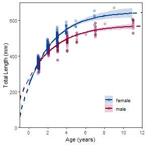
Some people may prefer to just see model fits. If so, then simply omit geom_point().
vbFitPlot2 <- ggplot() +
  geom_ribbon(data=preds2,aes(x=age,ymin=LCI,ymax=UCI,fill=sex),alpha=0.2) +
  geom_line(data=preds1,aes(y=fit,x=age,color=sex),size=1,linetype=2) +
  geom_line(data=preds2,aes(y=fit,x=age,color=sex),size=1) +
  scale_color_manual(values=c('#00429d', '#93003a'),
                     aesthetics=c("fill","color")) +
  scale_y_continuous(name="Total Length (mm)",limits=c(0,700),expand=c(0,0)) +
  scale_x_continuous(name="Age (years)",expand=c(0,0),
                     limits=c(-1,12),breaks=seq(0,12,2)) +
  theme_bw() +
  theme(panel.grid=element_blank(),
        legend.position=c(0.8,0.2),
        legend.title=element_blank())
vbFitPlot2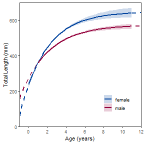
Multiple VBGFs in Separate Plots
An alternative to putting multiple VBGF trajectories in one plot is to separate them into individual plots. This is easily handled by including the “grouping” variable name within vars() within facet_wrap().4
vbFitPlot3 <- ggplot() +
  geom_ribbon(data=preds2,aes(x=age,ymin=LCI,ymax=UCI),alpha=0.2) +
  geom_point(data=w14T,aes(y=tl,x=age),alpha=0.25,size=2) +
  geom_line(data=preds1,aes(y=fit,x=age),size=1,linetype=2) +
  geom_line(data=preds2,aes(y=fit,x=age),size=1) +
  scale_y_continuous(name="Total Length (mm)",limits=c(0,700),expand=c(0,0)) +
  scale_x_continuous(name="Age (years)",expand=c(0,0),
                     limits=c(-1,12),breaks=seq(0,12,2)) +
  facet_wrap(vars(sex)) +
  theme_bw() +
  theme(panel.grid=element_blank())
vbFitPlot3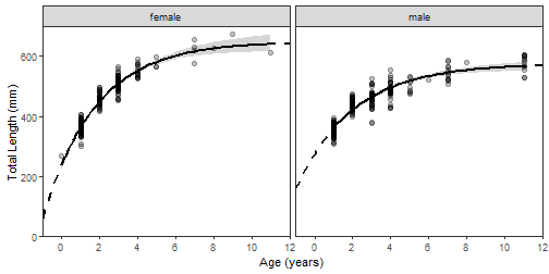
Faceting is more interesting when there are more “groups.” The plot below shows different VBGF fits across all available years for female Walleye from location “1.” The code is basically the same as above (i.e., strategically replacing sex with fyear and making sure to use the new data.frame).
wfT <- filter(WalleyeErie2,sex=="female",loc==1)

agesum <- group_by(wfT,year) %>%
  summarize(minage=min(age),maxage=max(age))

years <- unique(wfT$year)
nyears <- length(years)

cfs <- cis <- preds1 <- preds2 <- NULL

for (i in 1:nyears) {
  ## Loop notification (for peace of mind)
  cat(years[i],"Loop\n")
  ## Isolate year's data
  tmp1 <- filter(wfT,year==years[i])
  ## Fit von B to that year
  sv1 <- vbStarts(tl~age,data=tmp1)
  fit1 <- nls(tl~vb(age,Linf,K,t0),data=tmp1,start=sv1)
  ## Extract and store parameter estimates and CIs
  cfs <- rbind(cfs,coef(fit1))
  boot1 <- Boot(fit1)
  tmp2 <-  confint(boot1)
  cis <- rbind(cis,c(tmp2["Linf",],tmp2["K",],tmp2["t0",]))
  ## Predict mean lengths-at-age with CIs
  ##   preds1 -> across all ages
  ##   preds2 -> across observed ages only
  ages <- seq(-1,16,0.2)
  boot2 <- Boot(fit1,f=predict2)
  tmp2 <- data.frame(year=years[i],age=ages,
                     predict(fit1,data.frame(age=ages)),
                     confint(boot2))
  preds1 <- rbind(preds1,tmp2)
  tmp2 <- filter(tmp2,age>=agesum$minage[i],age<=agesum$maxage[i])
  preds2 <- rbind(preds2,tmp2)
}
## 2003 Loop
##
## Number of bootstraps was 631 out of 999 attempted
##
## Number of bootstraps was 615 out of 999 attempted## Warning in confint.boot(boot2): BCa method fails for this problem. Using 'perc' instead## 2004 Loop## Warning: Starting value for Linf is very different from the observed maximum
## length, which suggests a model fitting problem. See a Walford or
## Chapman plot to examine the problem. Consider either using the mean
## length for several of the largest fish (i.e., use 'oldAge' in
## 'methLinf=') or manually setting Linf in the starting value list
## to the maximum observed length.## 2005 Loop
##
## Number of bootstraps was 994 out of 999 attempted
##
## Number of bootstraps was 994 out of 999 attempted
## 2006 Loop
##
## Number of bootstraps was 998 out of 999 attempted
## 2007 Loop
## 2008 Loop
## 2009 Loop
## 2010 Loop
## 2011 Loop
## 2012 Loop
## 2013 Loop
## 2014 Looprownames(cfs) <- rownames(cis) <- years
colnames(cis) <- paste(rep(c("Linf","K","t0"),each=2),
rep(c("LCI","UCI"),times=2),sep=".")
colnames(preds1) <- colnames(preds2) <- c("year","age","fit","LCI","UCI")vbFitPlot4 <- ggplot() +
geom_ribbon(data=preds2,aes(x=age,ymin=LCI,ymax=UCI),alpha=0.2) +
geom_point(data=wfT,aes(y=tl,x=age),alpha=0.25,size=2) +
geom_line(data=preds1,aes(y=fit,x=age),size=1,linetype=2) +
geom_line(data=preds2,aes(y=fit,x=age),size=1) +
scale_y_continuous(name="Total Length (mm)",limits=c(0,800),expand=c(0,0)) +
scale_x_continuous(name="Age (years)",expand=c(0,0),
limits=c(-1,17),breaks=seq(0,16,2)) +
facet_wrap(vars(year),ncol=3) +
theme_bw() +
theme(panel.grid=element_blank())
vbFitPlot4## Warning: Removed 11 rows containing missing values (geom_path).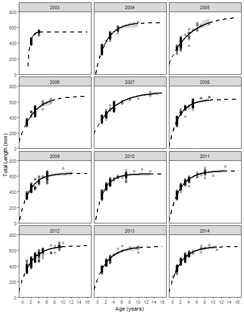
BONUS – Plots of Parameter Estimates
A bonus for keeping track of the parameter point and interval estimates through this entire post is to plot the estimates across years. I will leave this up to you to decipher, but note that the years must be added to the cfs and cis data.frames to make the plot shown here.
( cfs <- data.frame(year=years,cfs) )## year Linf K t0
## 2003 2003 540.1804 1.6843248 1.0770783
## 2004 2004 660.1222 0.3768720 -0.6210112
## 2005 2005 743.4416 0.1972271 -1.9791564
## 2006 2006 673.1494 0.2815995 -1.4618985
## 2007 2007 724.7986 0.2086957 -2.4787931
## 2008 2008 628.1655 0.3978859 -1.1359461
## 2009 2009 633.4864 0.4015328 -0.9812580
## 2010 2010 625.2466 0.4755051 -0.7492581
## 2011 2011 665.2861 0.3639903 -1.1207619
## 2012 2012 657.7450 0.3470683 -1.3561054
## 2013 2013 648.4110 0.3284681 -1.4754777
## 2014 2014 648.2084 0.3615400 -1.2836315( cis <- data.frame(year=years,cis) )## year Linf.LCI Linf.UCI K.LCI K.UCI t0.LCI t0.UCI
## 2003 2003 520.1261 557.3760 1.2259640 4.4428648 0.8088490 1.6059014
## 2004 2004 600.0443 698.6215 0.3104360 0.5082734 -0.8378565 -0.3766676
## 2005 2005 656.3570 999.5913 0.1072387 0.2762094 -3.0291481 -1.3073267
## 2006 2006 564.1173 799.5650 0.1815560 0.4936468 -2.0096527 -0.8289888
## 2007 2007 700.3794 756.5561 0.1823259 0.2379983 -2.8480065 -2.1156217
## 2008 2008 594.8101 682.2763 0.2723284 0.5447125 -1.7646474 -0.6974854
## 2009 2009 605.2833 670.3782 0.3308667 0.4758375 -1.2515718 -0.7680478
## 2010 2010 601.6751 644.2715 0.4212676 0.5569010 -0.9090219 -0.5701648
## 2011 2011 643.2538 692.5918 0.3084859 0.4245175 -1.3758088 -0.8968716
## 2012 2012 637.8887 680.3622 0.3082670 0.3940670 -1.5642523 -1.1527836
## 2013 2013 606.3430 683.4810 0.2787034 0.4037914 -1.7522694 -1.2037142
## 2014 2014 620.3367 687.8268 0.2998104 0.4270895 -1.5388048 -1.0630093p.Linfs <- ggplot() +
geom_point(data=cfs,aes(x=year,y=Linf)) +
geom_line(data=cfs,aes(x=year,y=Linf),color="gray80") +
geom_errorbar(data=cis,aes(x=year,ymin=Linf.LCI,ymax=Linf.UCI),width=0.3) +
scale_y_continuous(name=expression(L[infinity])) +
scale_x_continuous(name="Year",breaks=years) +
theme_bw() +
theme(panel.grid=element_blank(),
axis.text.x=element_text(angle=90,vjust=0.5))
p.Linfs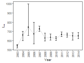
This is repeated for the other two parameters.
p.K <- ggplot() +
  geom_point(data=cfs,aes(x=year,y=K)) +
  geom_line(data=cfs,aes(x=year,y=K),color="gray80") +
  geom_errorbar(data=cis,aes(x=year,ymin=K.LCI,ymax=K.UCI),width=0.3) +
  scale_y_continuous(name="K") +
  scale_x_continuous(name=" ",breaks=years) +
  theme_bw() +
  theme(panel.grid=element_blank(),
        axis.text.x=element_text(angle=90,vjust=0.5))

p.t0 <- ggplot() +
  geom_point(data=cfs,aes(x=year,y=t0)) +
  geom_line(data=cfs,aes(x=year,y=t0),color="gray80") +
  geom_errorbar(data=cis,aes(x=year,ymin=t0.LCI,ymax=t0.UCI),width=0.3) +
  scale_y_continuous(name=expression(t[0])) +
  scale_x_continuous(name=" ",breaks=years) +
  theme_bw() +
  theme(panel.grid=element_blank(),
        axis.text.x=element_text(angle=90,vjust=0.5))
Which can then be neatly placed on top of each other with the patchwork package.
library(patchwork)
p.K / p.t0 / p.Linfs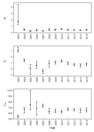
Final Thoughts
I am trying to post examples here as I learn ggplot2. My other ggplot2-related posts can be found here. I will post more about patchwork in future posts.
Footnotes
-
The parameter estimates and their confidence intervals are not needed to make the plots below; however, they are often of interest so I include them here. ↩
-
I inclued the notification in
cat()as it gives me peace of mind to see where the loop is at. This is useful here because this loop can take a while given the two sets of bootstraps. ↩ -
I used this resource to help choose two divergent colors that were “color-blind safe.” ↩
-
All
fill=sexandcolor=sexitems were removed from the previous code as leaving them in would result in each facet using a different color (which is redundant with the labels). ↩