Introduction
library(FSAdata) # for data
library(FSA)     # for vbFuns(), vbStarts(), confint.bootCase()
library(car)     # for Boot()
library(dplyr)   # for filter(), mutate()
library(ggplot2)
I am continuing to learn ggplot2 for elegant graphics. I often make a plot to illustrate the fit of a von Bertalanffy growth function to data. In general, I want this plot to have:
- Transparent points to address over-plotting of fish with the same length and age.
- A fitted curve with a confidence polygon over the range of observed ages.
- A fitted curve (without a confidence polygon) over a larger range than the observed ages (this often helps identify problematic fits).
Here I demonstrate how to produce such plots with lengths and ages of Lake Erie Walleye (Sander vitreus) captured during October-November, 2003-2014. These data are available in my FSAdata package and formed many of the examples in Chapter 12 of the Age and Growth of Fishes: Principles and Techniques book. My primary interest here is in the tl (total length in mm) and age variables (see here for more details about the data). I focus on female Walleye from location “1” captured in 2014 in this example.
data(WalleyeErie2)
wf14T <- dplyr::filter(WalleyeErie2,year==2014,sex=="female",loc==1)
The workflow below requires understanding the minimum and maximum observed ages.
agesum <- group_by(wf14T,sex) %>%
  summarize(minage=min(age),maxage=max(age))
agesum
## # A tibble: 1 x 3
## sex minage maxage
## <fct> <int> <int>
## 1 female 0 11
Fitting a von Bertalanffy Growth Function
Methods for fitting a von Bertalannfy growth function (VBGF) are detailed in my Introductory Fisheries Analyses with R book and in Chapter 12 of Age and Growth of Fishes: Principles and Techniques book. Briefly, a function for the typical VBGF is constructed with vbFuns()1.
( vb <- vbFuns(param="Typical") )## function(t,Linf,K=NULL,t0=NULL) {
## if (length(Linf)==3) { K <- Linf[[2]]
## t0 <- Linf[[3]]
## Linf <- Linf[[1]] }
## Linf*(1-exp(-K*(t-t0)))
## }
## <bytecode: 0x0000026cd7aa2768>
## <environment: 0x0000026ce4e1acc8>Reasonable starting values for the optimization algorithm may be obtained with vbStarts(), where the first argument is a formula of the form lengths~ages where lengths and ages are replaced with the actual variable names containing the observed lengths and ages, respectively, and data= is set to the data.frame containing those variables.
( f.starts <- vbStarts(tl~age,data=wf14T) )## $Linf
## [1] 645.2099
##
## $K
## [1] 0.3482598
##
## $t0
## [1] -1.548925The nls() function is typically used to estimate parameters of the VBGF from the observed data. The first argument is a formula that has lengths on the left-hand-side and the VBGF function created above on the right-hand-side. The VBGF function has the ages variable as its first argument and then Linf, K, and t0 as the remaining arguments (just as they appear here). Again, the data.frame with the observed lengths and ages is given to data= and the starting values derived above are given to start=.
f.fit <- nls(tl~vb(age,Linf,K,t0),data=wf14T,start=f.starts)The parameter estimates are extracted from the saved nls() object with coef().
coef(f.fit)## Linf K t0
## 648.208364 0.361540 -1.283632Bootstrapped confidence intervals for the parameter estimates are computed by giving the saved nls() object to Boot() and giving the saved Boot() object to confint().
f.boot1 <- Boot(f.fit)  # Be patient! Be aware of some non-convergence
confint(f.boot1)
## Bootstrap bca confidence intervals
##
## 2.5 % 97.5 %
## Linf 619.519302 686.5927399
## K 0.297934 0.4317571
## t0 -1.548261 -1.0503317
Preparing Predicted Values for Plotting
Predicted lengths-at-age from the fitted VBGF is needed to plot the fitted VBGF curve. The predict() function may be used to predict mean lengths at ages from the saved nls() object.
predict(f.fit,data.frame(age=2:7))## [1] 450.4495 510.4490 552.2448 581.3599 601.6415 615.7698What is need, however, is the predicted mean lengths at ages for each bootstrap sample, so that bootstrapped confidence intervals for each mean length-at-age can be derived. To do this with Boot(), predict() needs to be embedded into another function. For example, the function below does the same as predict() but is in a form that will work with Boot().
predict2 <- function(x) predict(x,data.frame(age=ages))
ages <- 2:7
predict2(f.fit)  # demonstrates same result as predict() above
## [1] 450.4495 510.4490 552.2448 581.3599 601.6415 615.7698Predicted mean lengths-at-age, with bootstrapped confidence intervals, can then be constructed by giving Boot() the saved nls() object AND the new prediction function in f=. The Boot() code will thus compute the predicted mean length at all ages between -1 and 12 in increments of 0.22. I extended the age range outside the observed range of ages as I want to see the shape of the curve nearer t0 and at older ages (to better see L∞).
ages <- seq(-1,12,by=0.2)
f.boot2 <- Boot(f.fit,f=predict2)  # Be patient! Be aware of some non-convergence
The vector of ages, the predicted mean lengths-at-age (from predict()), and the associated bootstrapped confidence intervals (from confint()) are placed into a data.frame for later use.
preds1 <- data.frame(ages,
                     predict(f.fit,data.frame(age=ages)),
                     confint(f.boot2))
names(preds1) <- c("age","fit","LCI","UCI")
headtail(preds1)
## age fit LCI UCI
## V1 -1.0 63.17547 12.18055 102.3627
## V2 -0.8 103.98483 62.48577 136.5450
## V3 -0.6 141.94750 108.01521 168.4213
## V64 11.6 642.05952 615.02952 672.9536
## V65 11.8 642.48843 615.36045 673.8122
## V66 12.0 642.88743 615.56480 674.5265For my purposes below, I also want predicted mean lengths only for observed ages. To make the code below cleaner, a new data.frame restricted to the observed ages is made here.
preds2 <- filter(preds1,age>=agesum$minage,age<=agesum$maxage)
headtail(preds2)
## age fit LCI UCI
## 1 0.0 240.6728 224.2408 253.8395
## 2 0.2 269.1007 256.7356 278.7312
## 3 0.4 295.5456 286.5712 302.3211
## 54 10.6 639.3815 613.6163 668.0091
## 55 10.8 639.9972 614.0103 669.1005
## 56 11.0 640.5700 614.2978 670.1147
Constructing the Plot
A ggplot2 often starts by defining data= and aes()thetic mappings in ggplot(). However, the data and aesthetics should not be set in ggplot in this application because information will be drawn from three data.frames – wf14T, preds, and preds2. Thus, the data and aesthetics will be set within specific geoms.
The plot begins with a polygon that encases the lower and upper confidence interval values for mean length at each age. This polygon is constructed with geom_ribbon() using preds2 (the confidence polygon will only cover observed ages) where the x-axis will be age and the minimum part of the y-axis will be LCI and the maximum part of the y-axis will be UCI. The fill color of the polygon is set with fill=.3
ggplot() +
  geom_ribbon(data=preds2,aes(x=age,ymin=LCI,ymax=UCI),fill="gray90")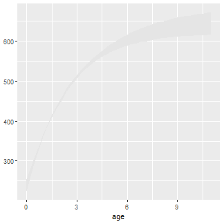
Observed lengths and ages in the wf14T data.frame were then added to this plot with geom_point(). The points are slightly larger than the default (with size=) and also with a fairly low transparency value to handle considerable over-plotting.
ggplot() +
  geom_ribbon(data=preds2,aes(x=age,ymin=LCI,ymax=UCI),fill="gray90") +
  geom_point(data=wf14T,aes(y=tl,x=age),size=2,alpha=0.1)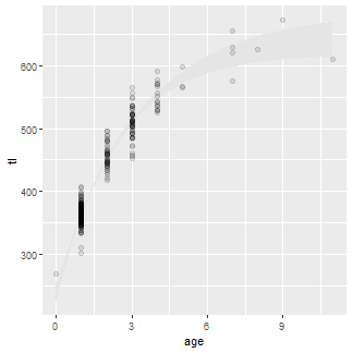
The fitted curve over the entire range of ages used above (i.e., using preds1) is added with geom_line(). A slightly thicker than default (size=) dashed (linetype=) line was used.
ggplot() +
  geom_ribbon(data=preds2,aes(x=age,ymin=LCI,ymax=UCI),fill="gray90") +
  geom_point(data=wf14T,aes(y=tl,x=age),size=2,alpha=0.1) +
  geom_line(data=preds1,aes(y=fit,x=age),size=1,linetype=2)
The fitted curve for just the observed range of ages (i.e., using preds2) is added using a solid line so that the dashed line for the observed ages is covered.
ggplot() +
  geom_ribbon(data=preds2,aes(x=age,ymin=LCI,ymax=UCI),fill="gray90") +
  geom_point(data=wf14T,aes(y=tl,x=age),size=2,alpha=0.1) +
  geom_line(data=preds1,aes(y=fit,x=age),size=1,linetype=2) +
  geom_line(data=preds2,aes(y=fit,x=age),size=1)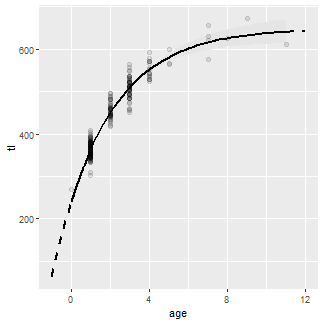
The y- and x-axes are labelled (name=), expansion factor for the axis limits is removed (expand=c(0,0)) so that the point (0,0) is in the corner of the plot, and the axis limits (limits=) and breaks (breaks=) are controlled using scale_y_continuous() and scale_x_continuous().
ggplot() +
  geom_ribbon(data=preds2,aes(x=age,ymin=LCI,ymax=UCI),fill="gray90") +
  geom_point(data=wf14T,aes(y=tl,x=age),size=2,alpha=0.1) +
  geom_line(data=preds1,aes(y=fit,x=age),size=1,linetype=2) +
  geom_line(data=preds2,aes(y=fit,x=age),size=1) +
  scale_y_continuous(name="Total Length (mm)",limits=c(0,700),expand=c(0,0)) +
  scale_x_continuous(name="Age (years)",expand=c(0,0),
                     limits=c(-1,12),breaks=seq(0,12,2))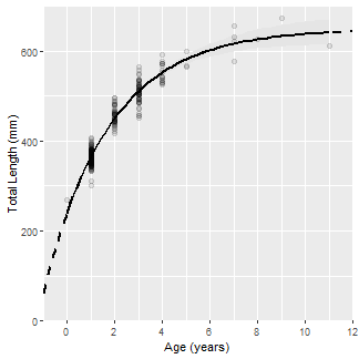
Finally, the classic black-and-white theme (primarily to remove the gray background) was used (theme_bw() and the grid lines were removed (panel.grid=).
vbFitPlot <- ggplot() +
  geom_ribbon(data=preds2,aes(x=age,ymin=LCI,ymax=UCI),fill="gray90") +
  geom_point(data=wf14T,aes(y=tl,x=age),size=2,alpha=0.1) +
  geom_line(data=preds1,aes(y=fit,x=age),size=1,linetype=2) +
  geom_line(data=preds2,aes(y=fit,x=age),size=1) +
  scale_y_continuous(name="Total Length (mm)",limits=c(0,700),expand=c(0,0)) +
  scale_x_continuous(name="Age (years)",expand=c(0,0),
                     limits=c(-1,12),breaks=seq(0,12,2)) +
  theme_bw() +
  theme(panel.grid=element_blank())
vbFitPlot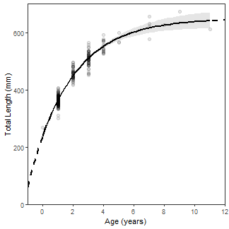
BONUS – Equation on Plot
Below is an undocumented bonus for how to put the equation of the best-fit VBGM on the plot. This is hacky so I would not expect it to be very general (e.g., it likely will not work across facets).
makeVBEqnLabel <- function(fit) {
  # Isolate coefficients (and control decimals)
  cfs <- coef(fit)
  Linf <- formatC(cfs[["Linf"]],format="f",digits=1)
  K <- formatC(cfs[["K"]],format="f",digits=3)
  # Handle t0 differently because of minus in the equation
  t0 <- cfs[["t0"]]
  t0 <- paste0(ifelse(t0<0,"+","-"),formatC(abs(t0),format="f",digits=3))
  # Put together and return
  paste0("TL==",Linf,"~bgroup('(',1-e^{-",K,"~(age",t0,")},')')")
}

vbFitPlot + annotate(geom="text",label=makeVBEqnLabel(f.fit),parse=TRUE,
                     size=4,x=Inf,y=-Inf,hjust=1.1,vjust=-0.5)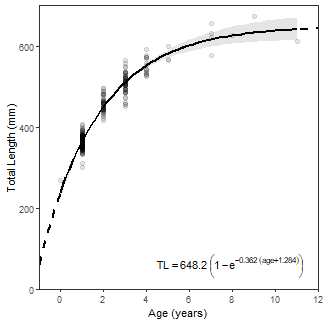
Final Thoughts
This post is likely not news to those of you that are familiar with ggplot2. However, I am trying to post some examples here as I learn ggplot2 in hopes that it will help others. My first post was here. In my next post I will demonstrate how to show von Bertalanffy curves for two or more groups.
Footnotes
-
Other parameterizations of the VBGF can be used with
param=invbFuns(). Parameterizations of the Gompertz, Richards, and Logistic growth functions are available inGompertzFuns(),RichardsFuns(), andlogisticFuns()of theFSApackage. See here for documentation. The Schnute four-parameter growth model is available inSchnute()and the Schnute-Richards five-parameter growth model is available inSchnuteRichards(). ↩ -
Reduce the value of
by=inseq()to make for a smoother VBGF curve when plotting later. ↩ -
This polygon will look better in the final plot when the gray background is removed. Also note that the polygon could be outlined by setting
color=to a color other than what is given infill=. ↩