A fishR user recently asked me
In the book that you published, I frequently use the stock-recruit curve code. The interface that shows both the Ricker/Beverton-Holt figure with the recruit per spawner to spawner figure (i.e., the dynamic plot for
srStarts()) has not been working for quite some time. Additionally, I can get the recruits versus spawner plot for the Beverton-Holt or Ricker curve with confidence bounds around the curve, but how do you do the same for the recruit per spawner to spawner curve?
Below I answer both questions. First, however, I load required packages …
library(FSA)      # srStarts, srFuns
library(FSAdata)  # PSalmonAK data
library(dplyr)    # %>%, filter, mutate, select
library(nlstools) # nlsBoot
… and obtain the same data (in PSalmonAK.csv available from here) used in the Stock-Recruitment chapter of my Introductory Fisheries Analyses with R (IFAR) book. Note that I created two new variables here: retperesc is the “recruits per spawner” and logretperesc is the natural log of the recruits per spawner variable.
pinks <- read.csv("data/PSalmonAK.csv") %>%
  filter(!is.na(esc),!is.na(ret)) %>%
  mutate(esc=esc/1000,ret=ret/1000,logret=log(ret),
         retperesc=ret/esc,logretperesc=log(retperesc)) %>%
  select(-SST)
headtail(pinks)
## year esc ret logret retperesc logretperesc
## 1 1960 1.418 2.446 0.894454 1.724965 0.5452066
## 2 1961 2.835 14.934 2.703640 5.267725 1.6615986
## 3 1962 1.957 10.031 2.305680 5.125703 1.6342676
## 28 1987 4.289 18.215 2.902245 4.246911 1.4461918
## 29 1988 2.892 9.461 2.247178 3.271438 1.1852298
## 30 1989 4.577 23.359 3.150982 5.103561 1.6299386Dynamic Plot Issue
The first question about the dynamic plot is due to a change in functionality in the FSA package since IFAR was published. The dynamicPlot= argument was removed because the code for that argument relied on the tcltk package, which I found difficult to reliably support. A similar, though more manual, approach is accomplished with the new fixed= and plot= arguments. For example, using plot=TRUE (without fixed=) will produces a plot of “recruits” versus “stock” with the chosen stock-recruitment model evaluated at the automatically chosen parameter starting values superimposed.
svR <- srStarts(ret~esc,data=pinks,type="Ricker",plot=TRUE)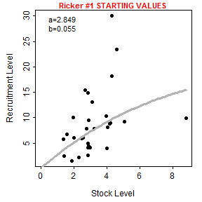
The user, however, can show the stock-recruitment model evaluated at manually chosen parameter starting values by including those starting values in a list that is supplied to fixed=. These values can be iteratively changed in subsequent calls to srStarts() to manually find starting values that provide a model that reasonably fits (by eye) the stock-recruit data.
svR <- srStarts(ret~esc,data=pinks,type="Ricker",plot=TRUE,
                fixed=list(a=4,b=0.15))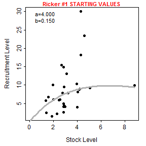
Note however that srStarts() no longer supports the simultaneously plotting of spawners versus recruits and recruits per spawner versus recruits.
Plot of Recruits per Spawner versus Spawners
The first way that I can imagine plotting recruits per spawners versus spawners with the fitted curve and confidence bands is to first follow the code for fitting the stock-recruit function to the stock and recruit data as described in IFAR. In this case, the stock-recruit function is fit on the log scale to adjust for a multiplicative error structure (as described in IFAR).
rckr <- srFuns("Ricker")
srR <- nls(logret~log(rckr(esc,a,b)),data=pinks,start=svR)
bootR <- nlsBoot(srR)
cbind(estimates=coef(srR),confint(bootR))
## estimates 95% LCI 95% UCI
## a 2.84924206 1.74768271 4.8435727
## b 0.05516673 -0.08443862 0.2158164As described in the book, the plot of spawners versus recruits is made by (i) constructing a sequence of “x” values that span the range of observed numbers of spawners, (ii) predicting the number of recruits at each spawner value using the best-fit stock-recruitment model, (iii) constructing lower and upper confidence bounds for the predicted number of recruits at each spawner value with the bootstrap results, (iv) making a schematic plot on which to put (v) a polygon for the confidence band, (vi) the raw data points, and (vii) the best-fit curve. The code below follows these steps and reproduces Figure 12.4 in the book.
x <- seq(0,9,length.out=199)        # many S for prediction
pR <- rckr(x,a=coef(srR))           # predicted mean R
LCI <- UCI <- numeric(length(x))

for(i in 1:length(x)) {             # CIs for mean R @ each S
  tmp <- apply(bootR$coefboot,MARGIN=1,FUN=rckr,S=x[i])
  LCI[i] <- quantile(tmp,0.025)
  UCI[i] <- quantile(tmp,0.975)
}
ylmts <- range(c(pR,LCI,UCI,pinks$ret))
xlmts <- range(c(x,pinks$esc))

plot(ret~esc,data=pinks,xlim=xlmts,ylim=ylmts,col="white",
     ylab="Returners (millions)",
     xlab="Escapement (millions)")
polygon(c(x,rev(x)),c(LCI,rev(UCI)),col="gray80",border=NA)
points(ret~esc,data=pinks,pch=19,col=col2rgbt("black",1/2))
lines(pR~x,lwd=2)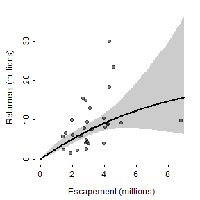
These results can be modified to plot recruits per spawner versus spawners by replacing the “recruits” in the code above with “recruits per spawner.” This is simple for the actual data as ret is simply replaced with retperesc. However, the predicted number of recruits (in pR) and the confidence bounds (in LCI and UCI) from above must be divided by the number of spawners (in x). As the / symbol has a special meaning in R formulas, this division must be contained within I() as when it appears in a formula (see the lines() code below). Of course, the y-axis scale range must also be adjusted. Thus, a plot of recruits per spawner versus spawners is produced from the previous results with the following code.
ylmts <- c(0.7,7)
plot(retperesc~esc,data=pinks,
     xlim=xlmts,ylim=ylmts,col="white",
     ylab="Returners/Escapement",
     xlab="Escapement (millions)")
polygon(c(x,rev(x)),c(LCI/x,rev(UCI/x)),col="gray80",border=NA)
points(retperesc~esc,data=pinks,pch=19,col=col2rgbt("black",1/2))
lines(I(pR/x)~x,lwd=2)
Alternatively, the Ricker stock-recruitment model could be reparameterized by dividing each side of the function by “spawners” such that the right-hand-side becomes “recruits per spawner” (this is a fairly typical reparameterization of the model). This model can be put into an R function, with model parameters then estimated with nonlinear regression similar to above. The results below show that the paramter point estimates are identical and the bootsrapped confidence intervals are similar to what was obtained above.
rckr2 <- function(S,a,b=NULL) {
  if (length(a)>1) { b <- a[[2]]; a <- a[[1]] }
  a*exp(-b*S)
}
srR2 <- nls(logretperesc~log(rckr2(esc,a,b)),data=pinks,start=svR)
bootR2 <- nlsBoot(srR2)
cbind(estimates=coef(srR2),confint(bootR2))
## estimates 95% LCI 95% UCI
## a 2.84924202 1.67734916 4.8613811
## b 0.05516673 -0.08776123 0.2040402With this, a second method for plotting recruits per spawner versus spawners is the same as how the main plot from the book was constructed but modified to use the results from this “new” model.
x <- seq(0,9,length.out=199)        # many S for prediction
pRperS <- rckr2(x,a=coef(srR2))     # predicted mean RperS
LCI2 <- UCI2 <- numeric(length(x))

for(i in 1:length(x)) {             # CIs for mean RperS @ each S
  tmp <- apply(bootR2$coefboot,MARGIN=1,FUN=rckr2,S=x[i])
  LCI2[i] <- quantile(tmp,0.025)
  UCI2[i] <- quantile(tmp,0.975)
}
ylmts <- range(c(pRperS,LCI2,UCI2,pinks$retperesc))
xlmts <- range(c(x,pinks$esc))

plot(retperesc~esc,data=pinks,xlim=xlmts,ylim=ylmts,col="white",
     ylab="Returners/Escapement",
     xlab="Escapement (millions)")
polygon(c(x,rev(x)),c(LCI2,rev(UCI2)),col="gray80",border=NA)
points(retperesc~esc,data=pinks,pch=19,col=col2rgbt("black",1/2))
lines(pRperS~x,lwd=2)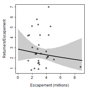
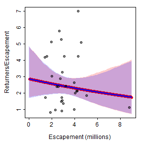
The two methods described above for plotting recruits per spawner versuse spawners are identical for the best-fit curve and nearly identical for the confidence bounds (slight differences likely due to the randomness inherent in bootstrapping). Thus, the two methods produce nearly the same visual.
plot(retperesc~esc,data=pinks,xlim=xlmts,ylim=ylmts,col="white",
     ylab="Returners/Escapement",
     xlab="Escapement (millions)")
polygon(c(x,rev(x)),c(LCI/x,rev(UCI/x)),col=col2rgbt("red",1/5),border=NA)
lines(I(pR/x)~x,lwd=6,col="red")
polygon(c(x,rev(x)),c(LCI2,rev(UCI2)),col=col2rgbt("blue",1/5),border=NA)
lines(pRperS~x,lwd=2,col="blue")
points(retperesc~esc,data=pinks,pch=19,col=col2rgbt("black",1/2))