Introduction
Recently I was tasked with estimating mean weights at age for data that contained no weights, but did contain lengths and ages (ages were from applying an age-length key). A weight-length relationship was available (derived from a smaller sample from the same population). A question arose about whether the weight-length relationship should be used to predict weights for individual fish and then summarized to estimate mean weights at age or whether the weight-length relationship should be applied to summarized mean lengths at age to estimate mean weights at age.
This issue has been addressed in the literature. Ricker (1975; page 211) states that the true mean weight is always greater, “of the order of 5%,” than the mean weight computed from the weight-length relationship with the mean length. Tesch (1971) suggested that the error in predicting mean weight at age with the weight-length relationship using mean length-at-age would be about 5-10%. In a simulation study, Nielsen and Schoch (1980) found that Tesch’s suggestion was too general and that error was less than 10% when the coefficient of variation (CV; standard deviation divided by mean) in lengths was less than 10% but could be substantially higher when the CV was higher, with the specific result dependent on the weight-length regression exponent (b). [Note that Nielsen and Schoch (1980) povide a nice geometric description of why this bias occurs.] Pienaar and Ricker (1968) and Beyer (1991) both suggested corrections to reduce the bias in the mean weight at age produced by the weight-length regression using the mean length.
In this post, I quickly explore the bias in using the weight-length regression to estimate mean weight at age from mean length at age. I then quickly explore the correction factors suggested by Beyer (1991).
This post requires the FSA and dplyr packages.
library(FSA)
library(dplyr)
I also set the random number seed to make the results reproducible.
set.seed(678394)Create A Sample of Data
I used the following code to create a very simple population that consisted of lengths, weights, and ages of fish. Lengths were modeled as normal distributions within each age-class. Weights were predicted directly from a known weight-length relationship without any error (in wt1) and with a small amount of error (in wt2). Modeling data in this way is simple, but at least somewhat realistic (Figure 1).
# Generate some lengths
ages <- 3:8
ns <- c(100,80,50,30,15,5)
mns <- c(300,450,525,560,575,590)
sds <- rep(30,length(mns))
lens <- NULL
for (i in 1:length(ages)) lens <- c(lens,rnorm(ns[i],mean=mns[i],sd=sds[i]))

# Parameters of a weight-length relationship
loga <- -13.5
b <- 3.2

# Compute weights from the W-L relationship, w/ & w/o error
df <- data.frame(age=rep(ages,ns),len=round(lens,0)) %>%
  mutate(wt1=round(exp(loga+b*log(len)),0),
         wt2=round(exp(loga+b*log(len)+rnorm(length(lens),mean=0,sd=0.1)),0))
headtail(df)
## age len wt1 wt2
## 1 3 289 103 110
## 2 3 315 135 131
## 3 3 284 97 93
## 278 8 583 971 1006
## 279 8 612 1134 848
## 280 8 582 966 1032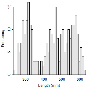
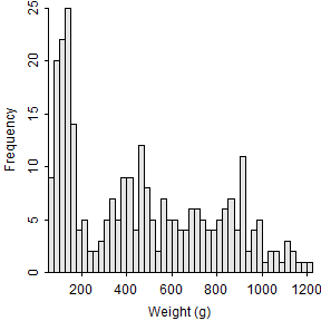
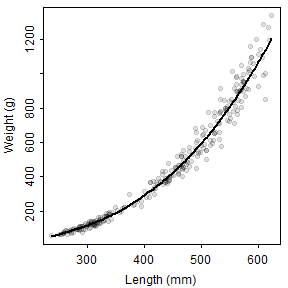
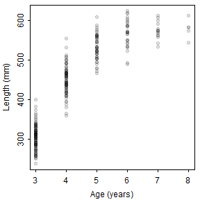
Figure 1: Histograms of lengths (upper left) and weights (upper right) and scatterplots of weight versus length (lower left) and length versus age (lower right). The line in the weight versus length scatterplot is the weights modeled without random error.
Explore the Bias
The first two lines below (using group_by() and summarize()) compute the mean length (mnlen) and true mean weight (i.e., the weight for individuals modeled above; true.mnwt) for the weights without any error for each age. The next line (using mutate()) computes the predicted mean weight at each age using the weight-length regression coefficients and the mean lengths just computed. The fourth line computes the percentage error between the predicted and true mean weights for each age.
sum1 <- group_by(df,age) %>%
  summarize(mnlen=mean(len),true.mnwt=mean(wt1)) %>%
  mutate(pr.mnwt=exp(loga+b*log(mnlen)),
         dif.mnwt=(pr.mnwt-true.mnwt)/true.mnwt*100) %>%
  as.data.frame()
The results from one example for the weights without any error show that the mean weight predicted from the mean length (pr.mnwt) is lower than the mean weight computed from individual weights predicted from individual lengths (true.mnwt; Table 1).
Table 1: Summary table using weights without any error and no correction for the predicted mean weights.
 age mnlen true.mnwt pr.mnwt dif.mnwt
   3   305       127     122    -3.47
   4   450       433     424    -2.17
   5   533       739     729    -1.24
   6   568       904     893    -1.22
   7   574       929     924    -0.48
   8   579       954     949    -0.52
Of course, weight-length relationships are not without error, so the weights with a small amount of random error were used to determine if the pattern of a negative bias when predicting mean weights from mean lengths persists with more realistic data. [Note that only a small error was added because the relationship between weight and length is very strong for most fishes. The r-squared for this relationship was a realistic 0.988.] Results from this one set of more realistic data showed a similar, though not as consistent, degree of negative bias when predicting mean weights from mean lengths (Table 2).
Table 2: Summary table using weights with a small amount of error and no correction for the predicted mean weights.
 age mnlen true.mnwt pr.mnwt dif.mnwt
   3   305       128     122    -4.37
   4   450       437     424    -3.09
   5   533       737     729    -1.03
   6   568       924     893    -3.36
   7   574       933     924    -0.95
   8   579       924     949     2.67
I then performed the analysis above 1000 times, keeping track of the percent error between the predicted weight and the true mean weight for each age for each sample. The results of this simulation suggest an average negative bias near 4% for age-3 fish and between about 1 and 2% for all older fish (Table 3). Note that the CV in length for each age varied between 0.6% and 13.0% in these simulations.
Table 3: Mean percentage difference in uncorrected predicted mean and true mean weights by age class for 1000 simulations.
age3 age4 age5 age6 age7 age8
-3.8 -2.0 -1.6 -1.4 -1.3 -1.1
Similar patterns were found using different values of the weight-length relationship exponent b (see Appendix). However, larger negative biases were observed as the standard deviation in lengths increased (see Appendix).
A Possible Correction
As noted above, Pienaar and Ricker (1968) and Beyer (1991) offered methods to reduce or eliminate the bias from using the weight-length regression to estimate mean weight at age from mean length at age. Beyer’s corrections were simple as they were based on the CV of lengths and the b coefficient from the weight-length regression. Beyer specifically offered three possible bias correcting factors for isometric growth and allometric growth assuming lognormal and normal distributions for lengths. Here I will only consider Beyer’s corrections for allometric growth with lognormal (i.e, Beyer’s equation 16) and normal (i.e., Beyer’s equation 18) distributions of lengths within age classes.
Beyer’s formulae are implemented by modifying group_by() and summarize() used previously. Specifically the standard deviation of lengths is calculated (in sdlen) so that the CV of lengths can be calculated (in cvlen). The correction factors are then computed (in cfn for the normal distribution and cfl for the lognormal distribution).
sum2a <- group_by(df,age) %>%
  summarize(mnlen=mean(len),sdlen=sd(len),
            true.mnwt=mean(wt2)) %>%
  mutate(cvlen=sdlen/mnlen,
         cfn=1+b*(b-1)/2*(cvlen^2),      # eqn 18
         cfl=(1+cvlen^2)^(b*(b-1)/2),    # eqn 16
         pr.mnwt=exp(loga)*mnlen^b,
         pr.mnwt.n=pr.mnwt*cfn,
         pr.mnwt.l=pr.mnwt*cfl,
         dif.mnwt=(pr.mnwt-true.mnwt)/true.mnwt*100,
         dif.mnwt.n=(pr.mnwt.n-true.mnwt)/true.mnwt*100,
         dif.mnwt.l=(pr.mnwt.l-true.mnwt)/true.mnwt*100) %>%
  as.data.frame()
These calculations were again repeated 1000 tiems and summarized in the bottom two rows of Table 4. These results suggest that the mean bias in predicted weights at age when corrected with a correction factor appear to only be on the order of a quarter to a half a percent. These corrections seems to perform fairly consistently across a few different values of the weight-length regression exponent b and standard deviations in lengths (see Appendix).
Table 4: Mean percentage difference in two types of corrected predicted mean and true mean weights by age class for 1000 simulations.
                    age3  age4  age5  age6  age7  age8
No correction      -3.83 -2.01 -1.55 -1.40 -1.25 -1.09
Normal (eqn 18)    -0.44 -0.49 -0.41 -0.40 -0.31 -0.18
Lognormal (eqn 16) -0.40 -0.48 -0.41 -0.39 -0.30 -0.18
Why Worry About This?
Why am I worried about this if the bias is on the order of 4% or less? First, for my application, we are estimating mean weight so that we can expand to total biomass. While a 4% error on an individual fish may seem inconsequential, that error can become quite important when expanded to represent total biomass, especially when it is a consistent negative bias.
So, why worry about correction factors when I can easily predict the weight for individual fish with the weight-length regression and then summarize these fish to get mean weight at age? In my situation, it appears that some of our mean lengths at age, and by extension mean weights at age, are poorly estimated because of small sample sizes at some ages. I am considering fitting a growth model (e.g., von Bertalanffy growth model) to the length-at-age data such that the fitted model can be used to predict mean lengths at age. The advantage of this is that information at other ages can be used to inform the calculation of mean length at an age. [The potential downside, of course, is that I would be prescribing a smooth curve to the growth trajectory.] If I can then estimate mean weights at age with minimal bias from the mean lengths at age from the growth model, then this could (I would need to test this) be beneficial in my situation.
Summary
Mean weights at age appear to be estimated with bias when a weight-length relationship is applied to mean lengths at age without any correction factor. The correction factors suggested by Beyer (1991) are easy to implement and seem to reduce the bias in predicted mean weights-at-age to near negligible levels. Thus, if mean weights at age cannot be predicted from individual fish, then it may be possible to get reasonable estimates from the weight-length relationship and mean lengths at age.
References
- Beyer, JE 1991. On length-weight relationships. Part 2. Computing mean weights from length statistics. FishByte 9:50-54.
- Nielsen, L.A. and W.F. Schoch. 1980. Errors in estimating mean weight and other statistics from mean length. Transactions of the American Fisheries Society 109:319-322.
- Pienaar, L.V. and W.E. Ricker. 1968. Estimating mean weight fomr length statistics. Journal of the Fisheries Research Board of Canada 25:2743-2747.
- Ricker, W.E. 1975. Computation and interpretation of biological statistics of fish populations. Bulletin of the Fisheries Research Board of Canada 25, Number 191.
- Tesch, F.W. 1971. Age and growth. Pages 98-126 in W.E. Ricker, editor. Methods for assessment of fish populations, 2nd edition. Blackwell Scientific Publications, Oxford, England.
Appendix: Summaries Using Different Values of b and SDs
Table 5: Summary table with everything the same but b=2.5.
                    age3  age4  age5  age6  age7  age8
No correction      -2.41 -1.17 -1.05 -0.95 -0.81 -0.83
Normal (eqn 18)    -0.59 -0.34 -0.44 -0.43 -0.30 -0.36
Lognormal (eqn 16) -0.58 -0.34 -0.44 -0.42 -0.29 -0.36
Table 6: Summary table with everything the same but b=3.0.
                    age3  age4  age5  age6  age7  age8
No correction      -3.32 -1.72 -1.41 -1.37 -1.14 -0.93
Normal (eqn 18)    -0.43 -0.41 -0.44 -0.53 -0.33 -0.16
Lognormal (eqn 16) -0.40 -0.41 -0.43 -0.52 -0.33 -0.16
Table 7: Summary table with everything the same but b=3.5.
                    age3  age4  age5  age6  age7  age8
No correction      -4.62 -2.35 -1.89 -1.74 -1.53 -1.34
Normal (eqn 18)    -0.45 -0.46 -0.48 -0.50 -0.34 -0.21
Lognormal (eqn 16) -0.38 -0.45 -0.47 -0.49 -0.34 -0.21
Table 8: Summary table with everything the same but SDs at 50.
                     age3  age4  age5  age6  age7  age8
No correction      -9.220 -4.58 -3.50 -3.13 -2.95 -2.27
Normal (eqn 18)    -0.402 -0.39 -0.42 -0.40 -0.36  0.15
Lognormal (eqn 16) -0.084 -0.32 -0.38 -0.37 -0.33  0.18
Table 9: Summary table with everything the same but SDs at 70.
                     age3  age4  age5  age6   age7  age8
No correction      -16.48 -8.18 -6.21 -5.42 -4.934 -4.10
Normal (eqn 18)     -0.45 -0.44 -0.36 -0.24  0.044  0.54
Lognormal (eqn 16)   0.71 -0.19 -0.23 -0.13  0.153  0.67