Explore Central Limit Theorem
The Central Limit Theorem (CLT), the specifics of which are in your module preparation notes, provides a mechanism for understanding what the sampling distribution of the sample means looks like. In this exercise, you will first identify what the CLT says the shape, center, and dispersion of the sampling distribution of sample means should look like for different sample sizes (n) from the known population shown below.
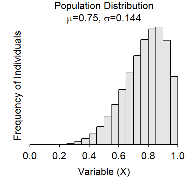
- What is the shape (normal or not), center (a specific value), and dispersion (a specific value) of the population shown in the plot above? [Note: Put specific symbols on the values for center and dispersion.]
- Based on the CLT record (in the table below) what you would expect the sampling distribution of the sample means to look like for samples of n=10, 25, and 50 taken from this population.
| Expected from CLT | |||
|---|---|---|---|
| Normal? | Center | Dispersion | |
| n=10 | |||
| n=25 | |||
| n=50 | |||
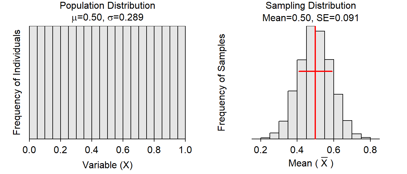
The sampling distribution of the sample means can be simulated by computing the means from many repeated samples from a population. The cltSim() function (with no arguments) efficiently computes sample means from many samples taken from a known population. The plots below were created with cltSim(). The histogram on the left below is the known population distribution (with μ & σ as shown). The histogram on the right is the distribution of sample means from 5000 samples of size n from the known population (i.e., a simulated sampling distribution).
In RStudio, a gear icon will be in the upper-left corner of this plot that will open a dialog box that allows you to change two shape parameters to alter the known population distribution. The population shown above uses shape1=6 and shape2=2. You should set those two sliders to those values and make sure that the population distribution (left plot) matches the population further above.
- Record what you observed about the sampling distribution of sample means (right plot) for each of n=10, 25, and 50 in the appropriate cells of the table below. [Use the “n” slider under the gear icon.]
Observed from cltSim()
|
|||
|---|---|---|---|
| Normal? | Center | Dispersion | |
| n=10 | |||
| n=25 | |||
| n=50 | |||
Evidence to support (or not) the CLT can be obtained by comparing what you expected to see (based on the CLT) for the sampling distribution of sample means to what you actually observed in the simulated distributions.
- Did each of your observations (second table) match your expectations (first table)?
- Do your observations on this exercise give you confidence in the CLT? Why or why not?