Coarse Woody Debris

Note:

Do NOT show the whole data frame, use str() instead.
For the categorical EDA simply comment on the most dominant characteristic or characteristics. In this case make sure to note that the medium exposure sites are much greater than the low exposure sites.
In both graphs the y-axis should be labeled with the frequency of INDIVIDUALS. In this case the “Frequency of CWD” or the “Frequency of Locations”.
Make sure you choose a binwidth that results in a decent look graph. If the bars are too few (i.e., wide) then use a smaller value, if the bars are too “spiky” (i.e., narrow) then use a larger value.

The vast majority of sites (82%) were exposed to medium levels of wind (as compared to low levels of wind).
The diameter of coarse woody debris in the north basin of Allequash Lake is strongly right-skewed with four potential outliers above 30 cm, a median (center) of 18 cm, and an IQR from Q1 of 16.2 to a Q3 of 20.8 cm. The median and IQR were used because of the strongly skew and potential outliers.

R Code and Results

> cwdobj <- read.csv("cwd.csv")

> str(cwdobj)

'data.frame':   50 obs. of  2 variables:
 $ diameter: int  21 15 18 23 18 17 19 17 15 22 ...
 $ exposure: chr  "med" "med" "med" "low" ...

> ( freq1 <- xtabs(~exposure,data=cwdobj) )

exposure
low med 
  9  41

> percTable(freq1)

exposure
low med 
 18  82

> ggplot(data=cwdobj,mapping=aes(x=exposure)) +
    geom_bar(color="black",fill="lightgray") +
    labs(x="Wind Expsure Category",y="Frequency of Sites") +
    scale_y_continuous(expand=expansion(mult=c(0,0.05))) +
    theme_NCStats()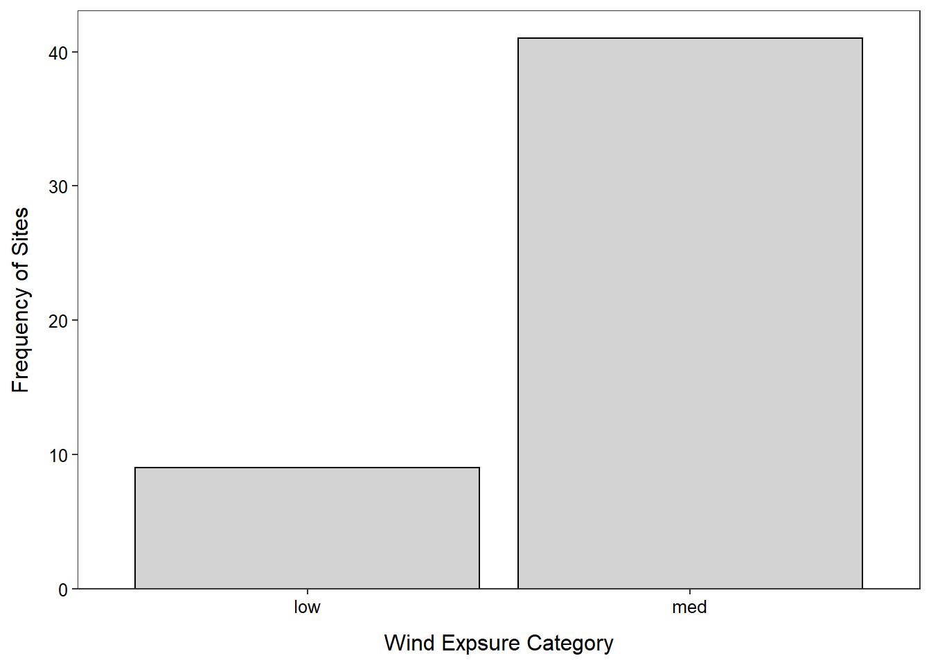

> Summarize(~diameter,data=cwdobj,digits=1)

     n   mean     sd    min     Q1 median     Q3    max 
  50.0   19.5    4.9   15.0   16.2   18.0   20.8   34.0

> ggplot(data=cwdobj,mapping=aes(x=diameter)) +
    geom_histogram(binwidth=1,boundary=0,color="black",fill="lightgray") +
    labs(x="CWD Diameter (cm)",y="Frequency of Sites") +
    scale_y_continuous(expand=expansion(mult=c(0,0.05))) +
    theme_NCStats()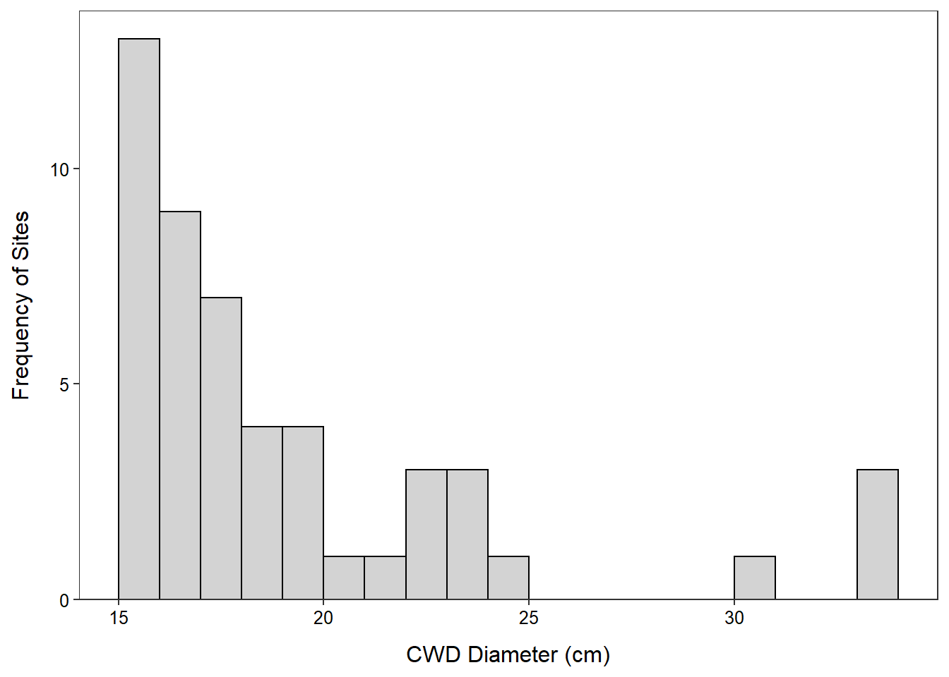

Brain Weights

Note:

Make sure you filter these data. Do NOT show the whole data frame, use str() instead.
Don’t say the shape is “normal”, you most likely mean that it is “symmetric.” Normal is very very specific and you cannot identify it by eye.
Make sure you choose a binwidth that results in a decent look graph. If the bars are too few (i.e., wide) then use a smaller value, if the bars are too “spiky” (i.e., narrow) then use a larger value.

The distribution of head sizes for the 20-46 age-group is very slightly right-skewed with no obvious outliers, a mean of 3675, and a standard deviation of 364.4. The mean and standard deviation were used because the shape was not strongly skewed and there were not obvious outliers.

R Code and Results

> bh <- read.csv("Brainhead.csv")

> ages20_46 <- filterD(bh,age.group=="20-46")
> str(ages20_46)

'data.frame':   110 obs. of  4 variables:
 $ head.size   : int  4512 3738 4261 3777 4177 3585 3785 3559 3613 3982 ...
 $ brain.weight: int  1530 1297 1335 1282 1590 1300 1400 1255 1355 1375 ...
 $ gender      : chr  "male" "male" "male" "male" ...
 $ age.group   : chr  "20-46" "20-46" "20-46" "20-46" ...

> Summarize(~head.size,data=ages20_46,digits=1)

     n   mean     sd    min     Q1 median     Q3    max 
 110.0 3675.3  364.4 2857.0 3440.0 3641.5 3897.0 4747.0

> ggplot(data=ages20_46,mapping=aes(x=head.size)) +
    geom_histogram(binwidth=100,boundary=0,color="black",fill="lightgray") +
    labs(x="Head Size (cm^3)",y="Frequency of Subjects") +
    scale_y_continuous(expand=expansion(mult=c(0,0.05))) +
    theme_NCStats()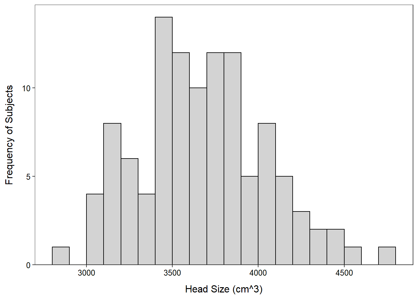

Water Usage

Note:

Do NOT show the whole data frame, use str() instead.
Don’t always just say what the most common value is. In this case the 6-10 min and 11-15 min groups are effectively equal so they should both be commented on.
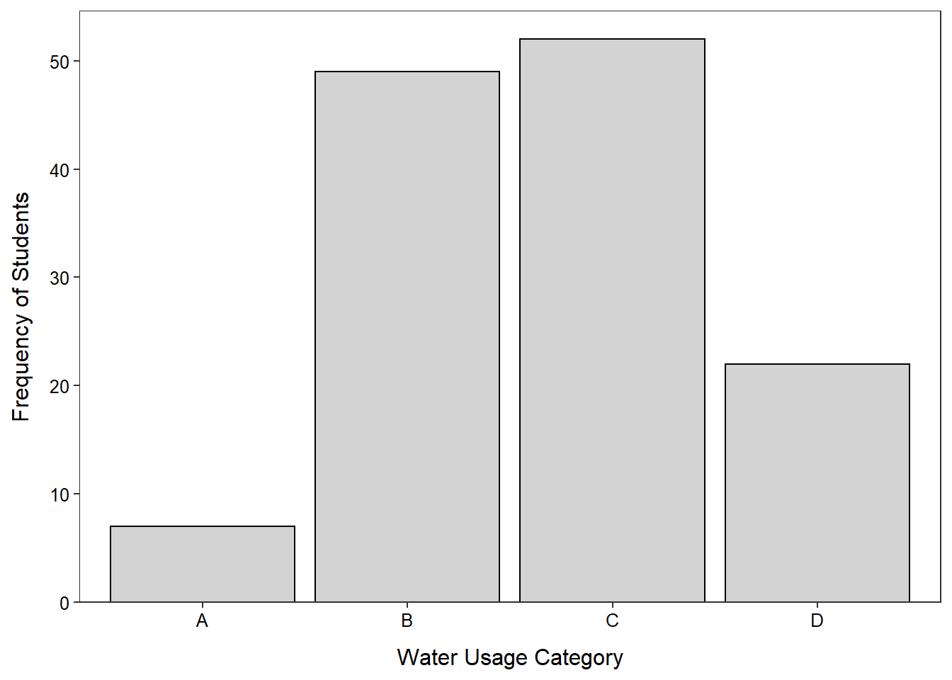
Don’t say “B” and “C”, say what those letters represent.

Most students either let the water run for 6-10 (37.7%) or 11-15 minutes (40.0%).

R Code and Results

> wtr <- read.csv("shower.csv")

> str(wtr)

'data.frame':   130 obs. of  1 variable:
 $ water.use: chr  "D" "C" "B" "B" ...

> ( freq1 <- xtabs(~water.use,data=wtr) )

water.use
 A  B  C  D 
 7 49 52 22

> percTable(freq1)

water.use
   A    B    C    D 
 5.4 37.7 40.0 16.9

> ggplot(data=wtr,mapping=aes(x=water.use)) +
    geom_bar(color="black",fill="lightgray") +
    labs(x="Water Usage Category",y="Frequency of Students") +
    scale_y_continuous(expand=expansion(mult=c(0,0.05))) +
    theme_NCStats()