Urban Runoff
- The equation of the best-fit line is IBI=37.8242-0.5136\(\times\)imp.
- If the percent of impervious surface increases by 1%, then the IBI score decreases by 0.51, on average.
- If the percent of impervious surface is 0, then the IBI score is 37.8, on average.
- The IBI score is predicted to be 22.4 when the percent of impervious surface is 30%.
- This question is an extrapolation and should not be answered (see plot below).
- The residual for an observed IBI score of 30 and a percent of impervious surface of 10% is 30-32.7=-2.7.
- The IBI will change by -25 slopes or 12.8 if the percentage of impervious surface is decreased by 20%. In other words the IBI will increase by 12.8 units.
- The correlation coefficient between IBI score and percent of impervious surface is -0.874.
- The proportion of variability in IBI scores that is explained by knowing the percent of impervious surface is 0.763.
- There appears to be homoscedasticity, but there is slight evidence of a curve suggesting that the relationship is nonlinear (see plot below).
R Code and Results
> d <- read.csv("IBI.csv")> ( lm1 <- lm(IBI~imp,data=d) )Coefficients:
(Intercept) imp
37.8242 -0.5136 > rSquared(lm1)[1] 0.7632712> ggplot(data=d,mapping=aes(x=imp,y=IBI)) +
geom_point(pch=21,color="black",fill="lightgray") +
labs(x="Percent Impervious Land",y="Benthic Index of Biotic Integrity") +
geom_smooth(method="lm",se=FALSE) +
theme_NCStats()`geom_smooth()` using formula 'y ~ x'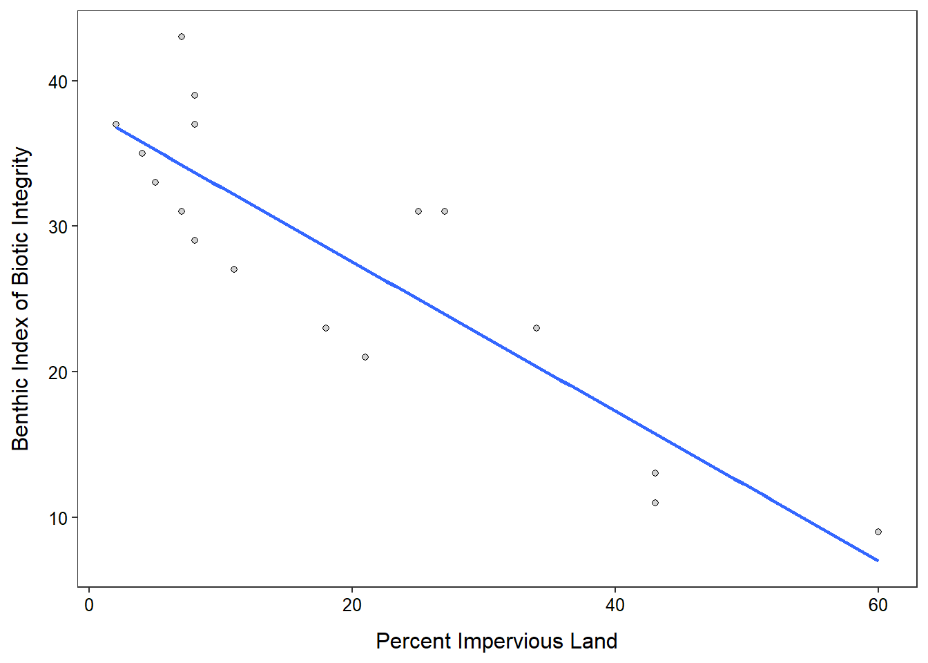
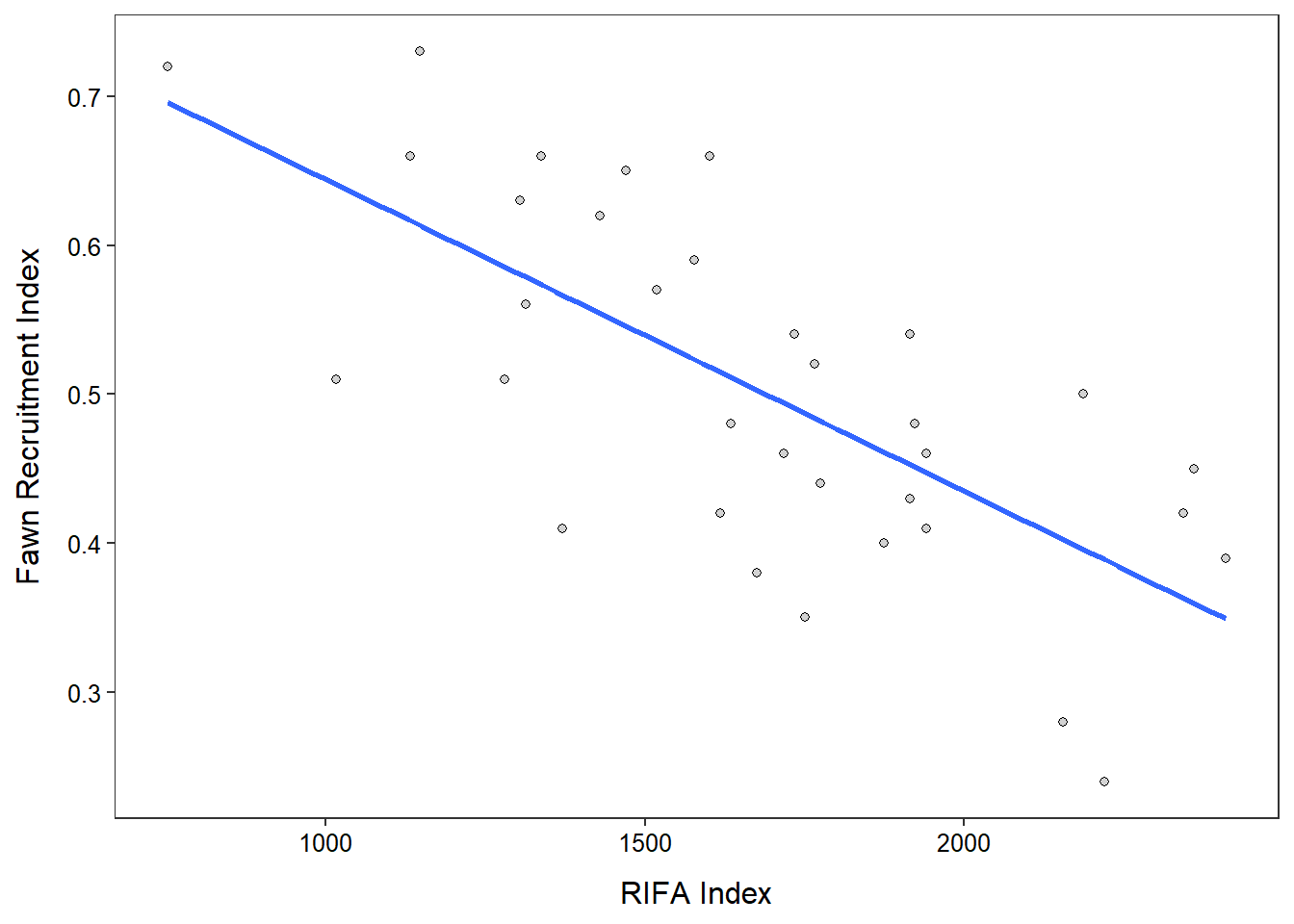
Red-Imported Fire Ants and Deer Fawns
- The response variable is the index of fawn recruitment. [Note that the index of fawn recruitment could depend on the RIFA index and the RIFA index is what is predicted or explained in the ensuing questions.]
- The explanatory variable is RIFA index.
- The best-fit line is fawnrec=-0.000209\(\times\)RIFA+0.854.
- The slope indicates that for every increase of one for the RIFA index the index of fawn recruitment will decrease by 0.000209, on average.
- The intercept indicates that if the RIFA index was zero, then the index of fawn recruitment would be 0.854, on average.
- If the RIFA index increased by 500 then the predicted index of fawn recruitment would decrease by 500 slopes or 0.105.
- This prediction should not be made as a RIFA index of 500 is outside the observed results for this variable (see plot below) and is, thus, an extrapolation.
- The predicted index of fawn recruitment if the RIFA index is 1700 is 0.498.
- The residual for an individual with a RIFA index of 2200 and a fawn recruitment index of 0.3 is 0.3-0.393=-0.093. Thus, this individual would have a lower fawn recruitment than the average for locations with a RIFA index of 2200.
- The correlation coefficient between RIFA and fawn recruitment indices is -0.700.
- The proportion of variability in the index of fawn recruitment that is explained by knowing the RIFA index is 0.49.
- I don’t have any strong concerns as the data appear linear (i.e., there is no obvious curve) and homoscedastic (i.e., there is no funnel or cone shape evident).
R Code and Results
> d <- read.csv("RIFA.csv")> ( lm1 <- lm(fawnrec~rifa,data=d) )Coefficients:
(Intercept) rifa
0.8536285 -0.0002093 > rSquared(lm1)[1] 0.4893269> ggplot(data=d,mapping=aes(x=rifa,y=fawnrec)) +
geom_point(pch=21,color="black",fill="lightgray") +
labs(x="RIFA Index",y="Fawn Recruitment Index") +
geom_smooth(method="lm",se=FALSE) +
theme_NCStats()`geom_smooth()` using formula 'y ~ x'