Climate Change Data
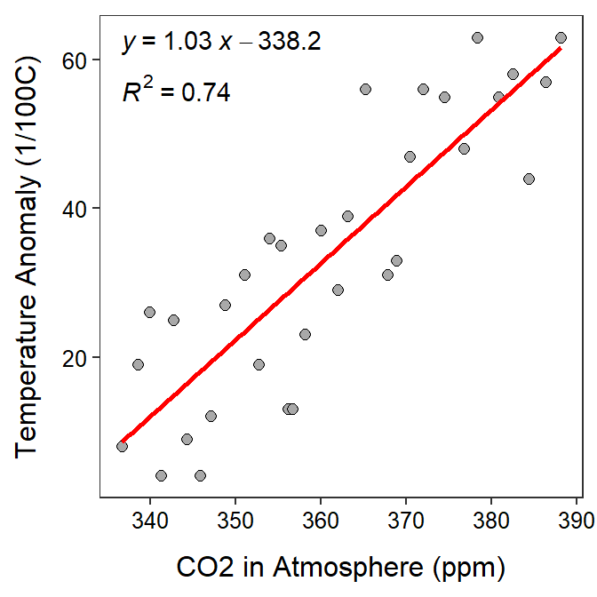
- The response variable is temperature anomaly.
- Temperature anomaly is the response variable because in the background we are told that “to determine if the variability in the temperature anomaly records can be reasonably explained by the CO2 values”. The response variable is the variable being explained. Additionally, the response variable is the variable to be predicted. In questions 6 and 7, it is clear that temperature anomaly is being predicted.
- Once you have identified the response variable that will make it clear which plot to use as the response variable is on the y-axis. Thus, in this case, use the left plot (reproduced above for convenience) and COMPLETELY IGNORE the other plot.
- The explanatory variable is the CO2 recordings.
- The explanatory variable is simply the “other” variable (i.e., not the response variable).
- The equation of the best fit line is TEMP=1.03CO2-338.2.
- This formula is written in Y=mX+b format and can be read directly from the equation on the plot.
- Make sure, however, that you replace Y and X with the names of the actual variables in the problem (TEMP and CO2 in this case).
- The slope indicates that for every 1 ppm increase in CO2 the temperature anomaly will increase 1.03 1/100oC, on average.
- The slope is the value that is multiplied by X or the explanatory variable.
- The slope interpretation is always how much Y changes for a one unit change in X; however, replace Y and X with the actual variable names.
- The best-fit line represents an average summary of the relationship between Y and X. Thus, the slope only represents an average change; therefore, you must include “on average” in your interpretation of the slope.
- The intercept indicates that the temperature anomaly will be -338.2 1/100oC on average when the CO2 in the atmosphere is 0 ppm.
- The intercept is the value in the equation not multiplied by X.
- The intercept will always be what the value of Y is when X is 0.
- You must include “on average” here for the same reason as described for the slope.
- The y-intercept will often not make sense because 0 is often not within the observed range of X values (as is clearly the case here).
- The temperature anomaly is predicted to be 32.6 1/100oC when the CO2 is 360 ppm.
- Before making a prediction make sure the value of X is within the range of observed X values. It is in this case so it is OK to make this prediction.
- This prediction is made by plugging 360 in for CO2 as shown below. \[ TEMP=1.03*360-338.2 \]
- The prediction should not be made as it is an extrapolation.
- Before making a prediction make sure the value of X is within the range of observed X values. It is NOT in this case so it is either NOT OK to make this prediction or you should acknowledge that the prediction could be wrong because it is an extrapolation.
- The residual if the temperature anomaly is 40 1/100oC and the CO2 is 380 ppm is -13.2 1/100oC.
- Computing a residuals requires predicting the value of Y at the given value of X. Thus, make sure the given value of X is with the observed range of X values. It is in this case so it is OK to make the prediction and proceed with the calculation.
- The predicted temperature anomaly for the given CO2 value is 53.2 1/100oC. This calculation is shown below.
- The residual is computed as the observed Y minus the predicted Y, as shown below. \[ RESIDUAL = 40 - 53.2 \]
\[ TEMP=1.03*380-338.2 \]
- The proportion of the variability in temperature anomaly that is explained by knowing the CO2 amount is 0.74.
- The words “proportion of variability … explained” can only mean the r2 value. Thus, simply report that value.
- The correlation coefficient between temperature anomaly and CO2 amount is 0.86.
- The correlation coefficient is symbolized with r, so simply take the square root of r2.
- However, if the slope had been negative you would need to add a negative sign to the square root result.
- If the CO2 amount were to increase by 20 ppm, then the temperature anomaly would be expected to increase by 20.6 1/100oC.
- This is largely another question about the slope. The slope says how much Y increases if X increases by 1. Thus, with this question we would expect Y to increase by 20 slopes as X increases by 20 units.
- I do not have any concerns about this best fit line because the form of the scatterplot is linear and the variability around the line is largely equal (i.e., it is homoscedastic). In other words, the form is NOT curved and the points are NOT funnel-shaped, so the regression assumptions are adequately met.
- With this question you should address the linearity and homoscedasticity assumptions. Linearity is met if the form is not curved. Homoscedasticity is met if the points don’t form a funnel of some sort..