Note:
- Don’t include the “mean” in the axis labels if the observed data are shown unless the observed data are means. In these examples the observed data are the frequency of the rattle for an INDIVIDUAL snake and the cumulative number of COVID cases for an INDIVIDUAL day. Thus, “mean” is not part of the variable and thus should not be in the axis labels. In the reading, the MEAN weight loss for a species of petrels was recorded so “mean” was part of the variable and is why it was included in the axis labels. If just the best-fit-line had been shown, without the observed points, then they y-axis would use “mean” because the lines represents a mean.
- When interpreting the slope on the transformed scale you say as “X” not “mean of X” increases by one and you say “mean of log of Y” not “log of mean of Y” (i.e., logging happened first, then the mean (i.e., best-fit line) was found).
- For the predictions using a confidence interval, make sure you say “mean” (you are predicting a mean value, not a value, for all individuals). However, for the predictions using a prediction interval, make sure you don’t say “mean” (you are predicting a value for a individual, not a mean for that individual).
Rattlesnake Rattling
- When transformed to the log-log scale, the form of the relationship appears to be linear and largely homoscedastic as there is no clear curve or funneling evident in the residual plot (shown below). The residuals do appear to be normal (Anderson-Darling p=0.7765) and there are not apparent outliers (p=0.0844).
- There is a significant relationship between log peak frequency and log weight of the rattlesnakes (ANOVA p<0.00005). The scatterplot with the best-fit line superimposed is shown below.
- The mean log peak frequency decreases between 0.099 and 0.188 for each unit increase in log weight of the rattlesnakes.
- The mean peak frequency is multiplied by a value between 0.829 and 0.906 for each 2.718 unit increase in weight of the rattlesnakes. In other words, the peak frequency decreases between 17.1 and 9.4% for each 2.718 unit increase in weight of the rattlesnakes.
- The peak frequency for a 454 g rattlesnake is between 4.978 and 7.760 kHz.
- The mean peak frequency for all 454 g rattlesnakes is between 5.895 and 6.553 kHz.
R Code and Results.
rs <- read.csv("https://raw.githubusercontent.com/droglenc/NCData/master/Rattlesnakes.csv")
lm.rs <- lm(freq~weight,data=rs)
assumptionCheck(lm.rs,lambday=0,lambdax=0)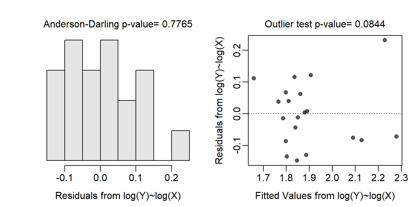
rs$logfreq <- log(rs$freq)
rs$logweight <- log(rs$weight)
lm.rst <- lm(logfreq~logweight,data=rs)
anova(lm.rst)
Analysis of Variance Table
Response: logfreq
Df Sum Sq Mean Sq F value Pr(>F)
logweight 1 0.48058 0.48058 45.628 2.494e-06
Residuals 18 0.18959 0.01053 ggplot(data=rs,mapping=aes(x=logweight,y=logfreq)) +
geom_point(pch=21,color="black",fill="lightgray") +
labs(x="log Weight",y="log Peak Frequency") +
theme_NCStats() +
geom_smooth(method="lm")`geom_smooth()` using formula 'y ~ x'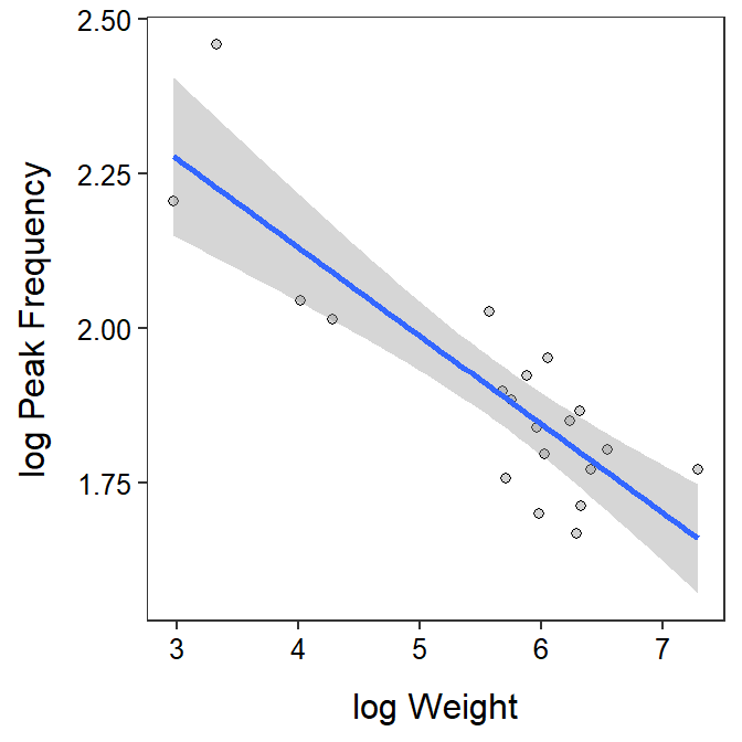
( cfs.rst <- cbind(Est=coef(lm.rst),confint(lm.rst)) ) ## log-log scale Est 2.5 % 97.5 %
(Intercept) 2.7039338 2.4483788 2.95948871
logweight -0.1433303 -0.1879095 -0.09875109exp(cfs.rst) ## back-transformed to original scale Est 2.5 % 97.5 %
(Intercept) 14.9383805 11.5695754 19.2881074
logweight 0.8664678 0.8286897 0.9059682nd <- data.frame(logweight=log(454))
( plog454 <- predict(lm.rst,newdata=nd,interval="prediction") ) # log scale fit lwr upr
1 1.827025 1.605015 2.049035exp(plog454) ## back-transformed to original scale fit lwr upr
1 6.21537 4.977936 7.760409( clog454 <- predict(lm.rst,newdata=nd,interval="confidence") ) # log scale fit lwr upr
1 1.827025 1.774123 1.879927exp(clog454) ## back-transformed to original scale fit lwr upr
1 6.21537 5.895112 6.553026
Initial COVID-19 Cases
- Assuming exponential growth implies that only the response variable, cumulative cases, should be transformed to the log scale. This was shown in the reading.
- This assumption removes the primary curve in the raw data (see residual plot below) but the data seems to have a bit of a cycle as shown in the scatterplot with best-fit line below. The log cumulative cases are below the best-fit line for about the first nine and last six days and generall above the line for the other days. However, there also seems to be a cycle about every 7 days or so … possibly due to reporting on weekends. Homoscedasticity, normality (Anderson-Darling p=0.1943), and no outlier (p>1) all appear to be largely met.
- There is a significant relationship between log cumulative cases and days since the 10th confirmed case (ANOVA p<0.00005). The scatterplot with the best-fit line superimposed is also shown below.
- The log cumulative cases increases between 0.242 and 0.262 each day.
- The cumulative cases increases by a multiple between 1.274 and 1.300 each day. In other words, the cumulative cases increases by between 27.4 and 30.0% each day.
- The cumulative cases are predicted to be between 970 and 2612 on day 20.
- The cumulative cases are predicted to be between 141897 and 428853 on day 40. One would have to assume continued exponential growth out to at least day 40 for this prediction to be meaningful.
R Code and Results.
cv <- read.csv("https://derekogle.com/NCMTH207/modules/ce/data/CovidUK.csv")
lm.cv <- lm(Cum_Cases~Days_Since_10,data=cv)
assumptionCheck(lm.cv,lambday=0)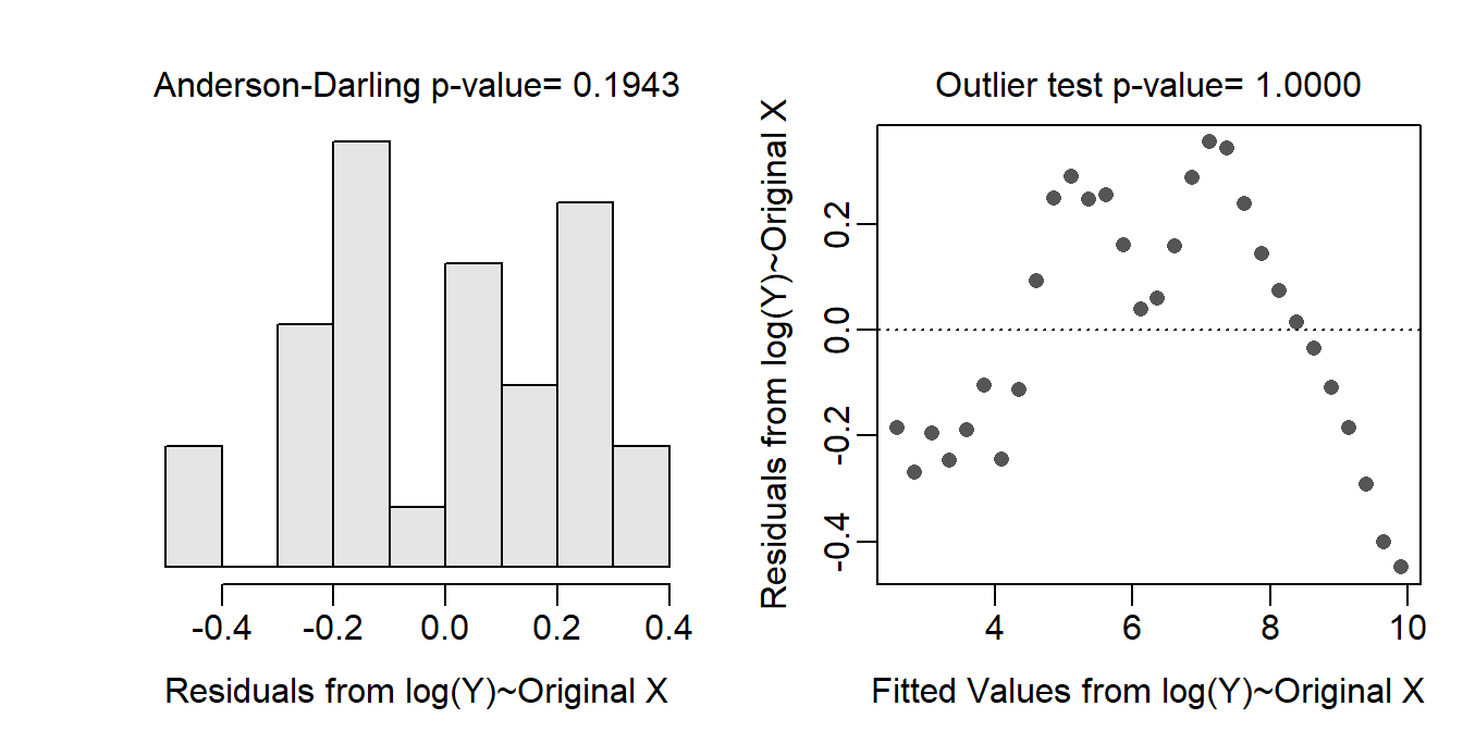
cv$logCum_Cases <- log(cv$Cum_Cases)ggplot(data=cv,mapping=aes(x=Days_Since_10,y=logCum_Cases)) +
geom_point(pch=21,color="black",fill="lightgray") +
labs(x="Days Since 10th Case Confirmed",y="log Cumulative Cases") +
theme_NCStats() +
geom_smooth(method="lm")`geom_smooth()` using formula 'y ~ x'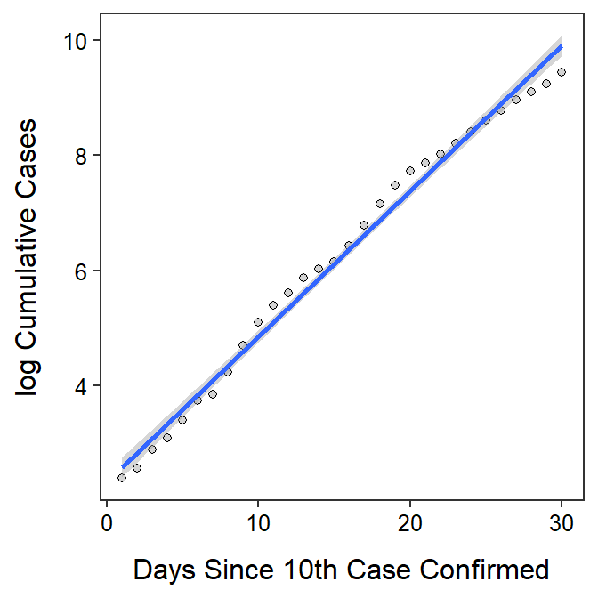
( cfs.cvt <- cbind(Est=coef(lm.rst),confint(lm.rst)) ) ## log-log scale Est 2.5 % 97.5 %
(Intercept) 2.7039338 2.4483788 2.95948871
logweight -0.1433303 -0.1879095 -0.09875109exp(cfs.cvt) ## back-transformed to original scale Est 2.5 % 97.5 %
(Intercept) 14.9383805 11.5695754 19.2881074
logweight 0.8664678 0.8286897 0.9059682nd <- data.frame(Days_Since_10=c(20,40))
( plogCC <- predict(lm.cvt,newdata=nd,interval="prediction") ) # log scale fit lwr upr
1 7.372669 6.877567 7.867771
2 12.415864 11.862859 12.968869exp(plogCC) ## back-transformed to original scale fit lwr upr
1 1591.877 970.2629 2611.738
2 246684.104 141897.2962 428852.762