Male-Female Birth Ratio

The df_Residual=n-2, thus n is df_Residual+2. In this case df_Residual=19 so n is 21.
The variance of the proportion of males among years ignoring any relationship with year is MS_Total=0.00000018(=\(\frac{0.00000356}{20}\)).
The variance of the proportion of males among years after taking into account the relationship between proportion of males and year is MS_Residual=0.00000007.
There is a significant relationship between the proportions of males and years (p=0.000014).
The p-values here (p=0.000014) and from the slope test on the previous exercise (p=0.000014) are the same. This occurs because the two tests effectively test the same null and alternative hypothesis. Furthermore, an F with 1 an 19 df is equal to the square of a t with 19 df.

R Code and Results.

br <- read.csv("BirthRatio.csv")

lm.br <- lm(propmale~year,data=br)
anova(lm.br)

Analysis of Variance Table

Response: propmale
          Df     Sum Sq    Mean Sq F value    Pr(>F)
year       1 2.2691e-06 2.2691e-06  33.399 1.439e-05
Residuals 19 1.2909e-06 6.7940e-08

summary(lm.br)

Coefficients:
              Estimate Std. Error t value Pr(>|t|)
(Intercept)  6.201e-01  1.860e-02  33.340  < 2e-16
year        -5.429e-05  9.393e-06  -5.779 1.44e-05

Residual standard error: 0.0002607 on 19 degrees of freedom
Multiple R-squared: 0.6374, Adjusted R-squared: 0.6183 
F-statistic:  33.4 on 1 and 19 DF,  p-value: 1.439e-05

Willow Flycatcher Migration

The df_Total=n-1, thus n is df_Total+1. In this case df_Total=21 so n is 22.
There is a significant relationship between wing length and day of migration (p=0.0444).
The F-ratio here (=4.5995) is the square of t test statistic for the slope from the previous exercise (=-2.1446²=4.5995). This occurs because the two tests effectively test the same null and alternative hypothesis. Furthermore, an F with 1 an 20 df is equal to the square of a t with 20 df.
The percent of the variability in wing length is explained by knowing the day of migration is 18.7 (i.e., 100r²).
The variance of wing length among birds after taking into account day of migration is MS_Residual=2.805.
The variance of wing length among birds ignoring any relationship with day of migration is MS_Total=3.286(=\(\frac{69.008}{21}\)).

R Code and Results.

wfc <- read.csv("https://raw.githubusercontent.com/droglenc/NCData/master/Flycatcher.csv")
lm.wfc <- lm(winglen~date,data=wfc)
summary(lm.wfc)

Coefficients:
            Estimate Std. Error t value Pr(>|t|)
(Intercept) 91.07024   10.74829   8.473 4.75e-08
date        -0.15576    0.07263  -2.145   0.0444

Residual standard error: 1.675 on 20 degrees of freedom
Multiple R-squared: 0.187,  Adjusted R-squared: 0.1463 
F-statistic: 4.599 on 1 and 20 DF,  p-value: 0.04445

rSquared(lm.wfc)

[1] 0.186974

anova(lm.wfc)

Analysis of Variance Table

Response: winglen
          Df Sum Sq Mean Sq F value  Pr(>F)
date       1 12.903 12.9026  4.5995 0.04445
Residuals 20 56.105  2.8053

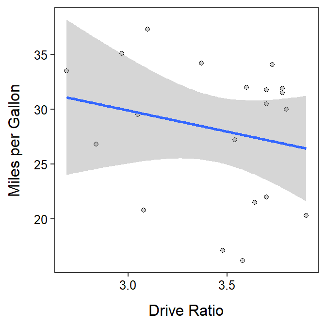
Car Drive Ratio and Gas Mileage

There is not a significant relationship between gas mileage and drive ratio for imported cars (p=0.3485).
The percent of the variability in gas mileage explained by knowing the drive ratio of an imported car is 4.9. Note that \(r^{2}\)=\(\frac{\text{SS}_{\text{Regression}}}{\text{SS}_{\text{Total}}}\)=\(\frac{37.309}{762.165}\)=0.049.
The variance of gas mileage among cars ignoring any relationship with drive ratio is MS_Total=40.114(=\(\frac{762.165}{19}\)).
The variance of gas mileage among cars after taking into account drive ratio is MS_Residual=40.270.
The plot is shown below.

R Code and Results.

gas <- read.csv("https://raw.githubusercontent.com/droglenc/NCData/master/CarMPG.csv")
gasI <- filter(gas,type=="Import")
lm.gas <- lm(mpg~drat,data=gasI)
summary(lm.gas)

Coefficients:
            Estimate Std. Error t value Pr(>|t|)
(Intercept)   41.501     13.928   2.980  0.00803
drat          -3.864      4.014  -0.963  0.34853

Residual standard error: 6.346 on 18 degrees of freedom
Multiple R-squared: 0.04895,    Adjusted R-squared: -0.003885 
F-statistic: 0.9265 on 1 and 18 DF,  p-value: 0.3485

rSquared(lm.gas)

[1] 0.0489514

anova(lm.gas)

Analysis of Variance Table

Response: mpg
          Df Sum Sq Mean Sq F value Pr(>F)
drat       1  37.31  37.309  0.9265 0.3485
Residuals 18 724.86  40.270

ggplot(data=gasI,mapping=aes(x=drat,y=mpg)) +  
  geom_point(pch=21,color="black",fill="lightgray") +  
  labs(x="Drive Ratio",y="Miles per Gallon") +  
  theme_NCStats() +  
  geom_smooth(method="lm")

`geom_smooth()` using formula 'y ~ x'