Note:

Any question about a “relationship” or “rate of change” will use some result about the slope. Questions of “significance” will use the slope p-value. Descriptions of the relationship will use the slope’s confidence interval.
When interpreting a negative slope, remove the negative and say “decreases.” Also flip your CI values so that it reads from the smallest value to the largest value.
Predictions of individuals use a prediction interval, whereas predictions of means for all individuals use a confidence interval.
Be thoughtful about your number of decimals … for means you generally only need 1 or 2 decimals more than the way the data were recorded … for p-values no more than 4 decimals is necessary.

Male-Female Birth Ratio

The variance of observations about the best-fit line is \(S_{Y|X}^{2}\)=0.000000068.
There is a statistical change in the proportion of male births in the U.S. over the study period because the slope is significantly less than 0 (p=0.000014). This slope would be how much the proportion of males changes per year. Thus, if it is less than zero then the proportion of of males is decreasing.
The proportion of males is decreasing at a rate between 0.000035 and 0.000074 per year, on average.
The p-value is so small even though the slope value is so small because the SE of the slope is even smaller. The SE of the slope is so small because the variability about the line is small and the overall scale of the proportion of males value is very small. The small p-value comes from a large t and the large t comes from the slope being much larger than the SE of the slope.

R Code and Results.

> br <- read.csv("BirthRatio.csv")

lm.br <- lm(propmale~year,data=br)
cbind(Est=coef(lm.br),confint(lm.br))

                      Est         2.5 %        97.5 %
(Intercept)  6.200857e-01  5.811580e-01  6.590134e-01
year        -5.428571e-05 -7.394606e-05 -3.462537e-05

summary(lm.br)

Coefficients:
              Estimate Std. Error t value Pr(>|t|)
(Intercept)  6.201e-01  1.860e-02  33.340  < 2e-16
year        -5.429e-05  9.393e-06  -5.779 1.44e-05

Residual standard error: 0.0002607 on 19 degrees of freedom
Multiple R-squared: 0.6374, Adjusted R-squared: 0.6183 
F-statistic:  33.4 on 1 and 19 DF,  p-value: 1.439e-05

Willow Flycatcher Migration

There is a relationsip between wing length and data of migration because the slope is significantly less than 0 (p=0.0444).
The slope (i.e., the relationship) means that for every increase of one day that the wing length decreases by between 0.004 and 0.307 mm, on average.
The predicted wing length for a bird that migrated on day 160 is between 62.1 and 70.2 mm. This is about a bird, so this uses a “prediction interval.”
The predicted mean wing length for all birds that migrated on day 160 is between 64.2 and 68.1 mm. This is about all birds, so this uses a “confidence interval.”
The prediction interval is wider because it needs to account for variability in placing the line and variability of individuals around the line, whereas the confidence interval is only concerned with variability in placement of the line.

R Code and Results.

wfc <- read.csv("https://raw.githubusercontent.com/droglenc/NCData/master/Flycatcher.csv")
lm.wfc <- lm(winglen~date,data=wfc)
cbind(Est=coef(lm.wfc),confint(lm.wfc))

                   Est      2.5 %        97.5 %
(Intercept) 91.0702393 68.6497096 113.490769073
date        -0.1557607 -0.3072602  -0.004261186

summary(lm.wfc)

Coefficients:
            Estimate Std. Error t value Pr(>|t|)
(Intercept) 91.07024   10.74829   8.473 4.75e-08
date        -0.15576    0.07263  -2.145   0.0444

Residual standard error: 1.675 on 20 degrees of freedom
Multiple R-squared: 0.187,  Adjusted R-squared: 0.1463 
F-statistic: 4.599 on 1 and 20 DF,  p-value: 0.04445

predict(lm.wfc,data.frame(date=160),interval="prediction")

       fit      lwr      upr
1 66.14853 62.13399 70.16307

predict(lm.wfc,data.frame(date=160),interval="confidence")

       fit      lwr      upr
1 66.14853 64.17111 68.12595

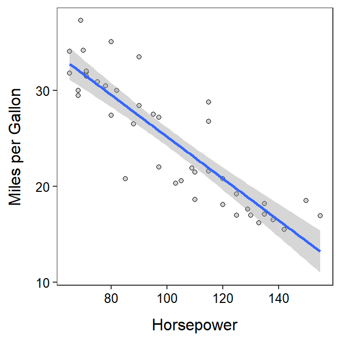
Car Horsepower and Gas Mileage

There is a significant relationship between mpg and horsepower because the slope is significantly less than 0 (p<0.00005).
The slope (i.e., the relationship) means that for every increase of one horsepower that the mpg decreases by between 0.181 and 0.255, on average.
The predicted mean mpg for all makes of car with horsepower of 110 is between 22.0 and 24.0. This is about all makes of cars, so this uses a “confidence interval.”
The predicted mpg for a make of car with a horsepower of 125 is between 13.3 and 26.1 mm. This is about a car, so this uses a “prediction interval.”
The predicted mpg for makes of cars with horsepowers of 125 and 126 is 19.724 and 19.506, respectively. Horsepowers of 125 and 126 represent an increase of one horsepower, so the difference between the two predictions (=19.506-19.724=-0.218) is the same as the slope (-0.218).
The graphic is shown below.

R Code and Results.

gas <- read.csv("https://raw.githubusercontent.com/droglenc/NCData/master/CarMPG.csv")
lm.gas <- lm(mpg~hp,data=gas)
cbind(Est=coef(lm.gas),confint(lm.gas))

                   Est      2.5 %    97.5 %
(Intercept) 46.9265926 43.0424051 50.810780
hp          -0.2176221 -0.2545932 -0.180651

summary(lm.gas)

Coefficients:
            Estimate Std. Error t value Pr(>|t|)
(Intercept) 46.92659    1.92184   24.42  < 2e-16
hp          -0.21762    0.01829  -11.90 1.03e-14

Residual standard error: 3.096 on 40 degrees of freedom
Multiple R-squared: 0.7796, Adjusted R-squared: 0.7741 
F-statistic: 141.5 on 1 and 40 DF,  p-value: 1.027e-14

predict(lm.gas,data.frame(hp=125),interval="prediction")

       fit      lwr      upr
1 19.72383 13.33395 26.11371

predict(lm.gas,data.frame(hp=110),interval="confidence")

       fit      lwr      upr
1 22.98816 21.97567 24.00066

predict(lm.gas,data.frame(hp=c(125,126)),interval="confidence")

       fit      lwr      upr
1 19.72383 18.43135 21.01631
2 19.50621 18.18886 20.82355

ggplot(data=gas,mapping=aes(x=hp,y=mpg)) +  
  geom_point(pch=21,color="black",fill="lightgray") +  
  labs(x="Horsepower",y="Miles per Gallon") +  
  theme_NCStats() +  
  geom_smooth(method="lm")

`geom_smooth()` using formula 'y ~ x'