R Code and Results
> predProb <- function(x,alpha,beta) exp(alpha+beta*x)/(1+exp(alpha+beta*x))
> predX <- function(p,alpha,beta) (log(p/(1-p))-alpha)/beta
> Ruffe <- read.csv("https://raw.githubusercontent.com/droglenc/NCData/master/RuffeLarvalDiet.csv")
> Ruffe <- filter(Ruffe,loc=="Allouez")
> Ruffe$daph01 <- ifelse(Ruffe$o.daph=="Y",1,0)
> glm.Ruffe <- glm(daph01~len,data=Ruffe,family=binomial)
> anova(glm.Ruffe,test="LRT")
Analysis of Deviance Table

Model: binomial, link: logit

Response: daph01

Terms added sequentially (first to last)

     Df Deviance Resid. Df Resid. Dev  Pr(>Chi)
NULL                   163    218.467
len   1   130.81       162     87.659 < 2.2e-16
> boot.Ruffe <- car::Boot(glm.Ruffe)
> cbind(Est=coef(glm.Ruffe),confint(boot.Ruffe,type="perc"))
                   Est      2.5 %    97.5 %
(Intercept) -10.711628 -15.934001 -8.322682
len           1.311943   1.007326  1.953905
> nd <- data.frame(len=6)
> ( lodds6 <- predict(glm.Ruffe,newdata=nd) )
       1
-2.83997
> exp(lodds6)
         1
0.05842739
> ( prob6 <- predict(glm.Ruffe,newdata=nd,type="response") )
         1
0.05520208
> prob6.boot <- predProb(6,boot.Ruffe$t[,1],boot.Ruffe$t[,2])
> ( prob6.ci <- quantile(prob6.boot,probs=c(0.025,0.975),type=1) )
      2.5%      97.5%
0.01237052 0.10864974
> x50.boot <- predX(0.5,boot.Ruffe$t[,1],boot.Ruffe$t[,2])
> ( x50.ci <- quantile(x50.boot,probs=c(0.025,0.975),type=1) )
    2.5%    97.5%
7.722297 8.586595
> x90.boot <- predX(0.9,boot.Ruffe$t[,1],boot.Ruffe$t[,2])
> ( x90.ci <- quantile(x90.boot,probs=c(0.025,0.975),type=1) )
     2.5%     97.5%
 9.141231 10.546048
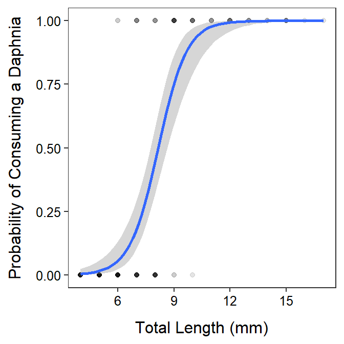
> ggplot(data=Ruffe,mapping=aes(x=len,y=daph01)) +
    geom_point(alpha=0.1) +
    geom_smooth(method="glm",method.args=list(family=binomial)) +
    labs(x="Total Length (mm)",y="Probability of Consuming a Daphnia") +
    theme_NCStats()