Nurse Wages
Note:
- Make sure to include the \(\mu\) part on the left-hand-side of yoru models.
- The hypotheses for the parallel lines test are:
- HA \(\mu_{WAGE|EXPER,MALE} = \alpha+\beta EXPER+\delta_{1}MALE+\gamma_{1}EXPER:MALE\).
- H0 \(\mu_{WAGE|EXPER,MALE} = \alpha+\beta EXPER+\delta_{1}MALE\).
- The hypotheses for the coincident lines test are:
- HA \(\mu_{WAGE|EXPER,MALE} = \alpha+\beta EXPER+\delta_{1}MALE\).
- H0 \(\mu_{WAGE|EXPER,MALE} = \alpha+\beta EXPER\).
- The hypotheses for the relationship test are:
- HA \(\mu_{WAGE|EXPER,MALE} = \alpha+\beta EXPER\).
- H0 \(\mu_{WAGE|EXPER,MALE} = \alpha\).
Turtle Nesting Ecology
Note:
- Make sure to include the \(\mu\) part on the left-hand-side of yoru models.
- The parallel lines test indicates that ALL of the lines are statistically parallel.
- The coincident lines test indicates that SOME of the lines are not coincident.
- When plotting the lines without any data then the y-axis label should include “mean.”
- The models for parallel lines test are as follows:
- HA: \(\mu_{CSIZE|CCL,\cdots} = \alpha+\beta CCL+\)\(\delta_{1}IO+\delta_{2}RS+\delta_{3}+\delta_{4}WA+\) \(\gamma_{1}CCL:IO+\gamma_{2}CCL:RS+\gamma_{3}CCL:CO+\gamma_{4}CCL:WA\).
- H0: \(\mu_{CSIZE|CCL,\cdots} = \alpha+\beta CCL+\)\(\delta_{1}IO+\delta_{2}RS+\delta_{3}+\delta_{4}WA\).
- The models for coincident lines test are as follows:
- HA: \(\mu_{CSIZE|CCL,\cdots} = \alpha+\beta CCL+\)\(\delta_{1}IO+\delta_{2}RS+\delta_{3}+\delta_{4}WA\).
- H0: \(\mu_{CSIZE|CCL,\cdots} = \alpha+\beta CCL\).
- The lines appear to be parallel across all regions (p=0.1192). Thus, the relationship between clutch size and curved carapace length does NOT differ among the regions.
- The intercepts appear to differ among some of the regions (p<0.00005). Thus, the mean clutch size at the same curved carapace length, no matter what that carapace length is, differs among some regions.
- There does appear to be a significant relationship between clutch size and curved carapace length (p<0.00005).
R Code and Results
ht <- read.csv("https://raw.githubusercontent.com/droglenc/NCData/master/HawksbillTurtles.csv")
ht$Region <- factor(ht$Region,
                    levels=c("Arabian Gulf","Indian Ocean","Red Sea",
                             "Caribbean","West Atlantic"))
ivr.ht <- lm(Clutch.Size~CCL+Region+CCL:Region,data=ht)
anova(ivr.ht)
Analysis of Variance Table
Response: Clutch.Size
Df Sum Sq Mean Sq F value Pr(>F)
CCL 1 246757 246757 526.8775 < 2.2e-16
Region 4 22045 5511 11.7675 5.266e-09
CCL:Region 4 3461 865 1.8472 0.1192
Residuals 368 172349 468 ggplot(data=ht,mapping=aes(x=CCL,y=Clutch.Size,color=Region)) +
labs(x="Curved Carapace Length (cm)",y="Clutch Size") +
theme_NCStats() +
geom_smooth(method="lm",se=FALSE)`geom_smooth()` using formula 'y ~ x'Warning: Removed 140 rows containing non-finite values (stat_smooth).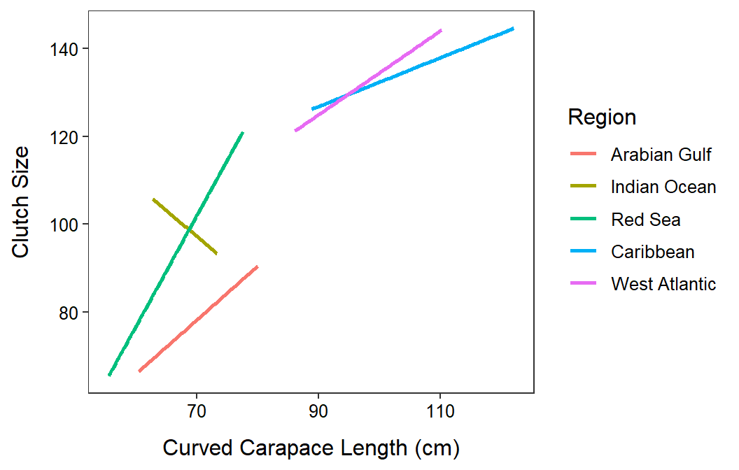
Water Quality Near a Gold Mine
Analysis of Variance Table

Response: phosp
              Df  Sum Sq Mean Sq F value    Pr(>F)
distance       1  8863.5  8863.5 48.0590 1.763e-09
type           2  3135.0  1567.5  8.4992 0.0005016
distance:type  2     5.0     2.5  0.0137 0.9864185
Residuals 69 12725.7 184.4 - The models for parallel lines test are as follows:
- HA: \(\mu_{P|DIST,\cdots} = \alpha+\beta DIST+\)\(\delta_{1}DP+\delta_{2}SP+\) \(\gamma_{1}DIST:DP+\gamma_{2}DIST:SP\).
- H0</sub: \(\mu_{P|DIST,\cdots} = \alpha+\beta DIST+\)\(\delta_{1}DP+\delta_{2}SP\).
- The models for coincident lines test are as follows:
- HA: \(\mu_{P|DIST,\cdots} = \alpha+\beta DIST+\)\(\delta_{1}DP+\delta_{2}SP\).
- H0: \(\mu_{P|DIST,\cdots} = \alpha+\beta DIST\).
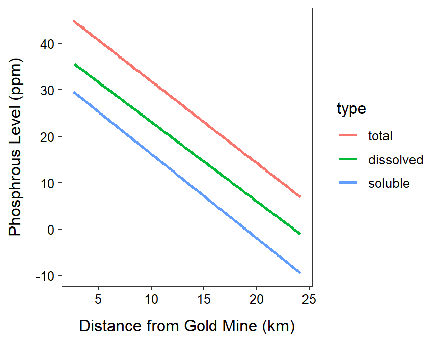
- The lines appear to be parallel across all three types of phosphorous (p=0.9864). Thus, the relationship between phosphorous level and distance from the gold mine does NOT differ among phosphorous types.
- The intercepts appear to differ among some of the phosphorous types (p=0.0005). Thus, the mean phosphorous level at the same distance from the gold mine, no matter what that distance is, differs among phosphorous types
- There does appear to be a significant relationship between phosphorous level and distance from the gold mine (p<0.00005).
R Code and Results
gm <- read.csv("http://derekogle.com/NCMTH207/modules/ce/data/GoldMine.csv")
gm$type <- factor(gm$type,levels=c("total","dissolved","soluble"))
ivr.gm <- lm(phosp~distance+type+distance:type,data=gm)
anova(ivr.gm)
Analysis of Variance Table
Response: phosp
Df Sum Sq Mean Sq F value Pr(>F)
distance 1 8863.5 8863.5 48.0590 1.763e-09
type 2 3135.0 1567.5 8.4992 0.0005016
distance:type 2 5.0 2.5 0.0137 0.9864185
Residuals 69 12725.7 184.4 ggplot(data=gm,mapping=aes(x=distance,y=phosp,color=type)) +
labs(x="Distance from Gold Mine (km)",y="Phosphrous Level (ppm)") +
theme_NCStats() +
geom_smooth(method="lm",se=FALSE)`geom_smooth()` using formula 'y ~ x'