Nurse Wages

The ultimate full model is \(\mu_{WAGE|EXPER,MALE} = \alpha+\beta EXPER+\delta_{1}MALE+\gamma_{1}EXPER:MALE\) where \(WAGE\) is the earned wage and \(EXPER\) is the years of experience.
Table shown below

Gender	MALE	Sub-Model (\(\mu_{WAGE\|EXPER}=\))
female	0	\(\alpha+\beta EXPER\)
male	1	\((\alpha+\delta_{1})+(\beta+\gamma_{1})EXPER\)

Meanings of the parameters are below.

\(\alpha\): y-intercept of female nurses (reference group).
\(\beta\): slope of female nurses (reference group).
\(\delta_{1}\): difference in y-intercept from male to female nurses.
\(\gamma_{1}\): difference in slope from male to female nurses.

I would expect \(\beta\) to be positive because if wages increases with experience then I would expect a positive relationship or slope.
I would expect \(\gamma_{1}\) to be negative because if a slower rate means a shallower or smaller slope; thus, if males have a smaller slope then \(\gamma_{1}\) must be negative.
I would expect \(\delta_{1}\) to be zero because the mean wage with no experience describes the y-intercept. If there is no difference in mean wage with no experience for males and females then they have the same intercept or no difference in intercpet, so \(\delta_{1}\)=0.
I would expect \(\delta_{1}\) to be positive because the descriptions states that the lines are parallel (i.e., \(\gamma_{1}\)=0) and the male line is always above the female line, incluing at the y-intercept.

Turtle Nesting Ecology

The ultimate full model is \(\mu_{CSIZE|CCL,\cdots} = \alpha+\beta CCL+\)\(\delta_{1}IO+\delta_{2}RS+\delta_{3}+\delta_{4}WA+\) \(\gamma_{1}CCL:IO+\gamma_{2}CCL:RS+\gamma_{3}CCL:CO+\gamma_{4}CCL:WA\) where \(CSIZE\) is clutch size, \(CCL\) is the curved carapace length, and the other variables were defined on the previous assignment.
Table shown below

Region	IO	RS	CO	WA	Sub-Model (\(\mu_{CSIZE\|CCL}=\))
Arabian Gulf	0	0	0	0	\(\alpha+\beta CCL\)
Indian Ocean	1	0	0	0	\((\alpha+\delta_{1})+(\beta+\gamma_{1})CCL\)
Red Sea	0	1	0	0	\((\alpha+\delta_{2})+(\beta+\gamma_{2})CCL\)
Caribbean	0	0	1	0	\((\alpha+\delta_{3})+(\beta+\gamma_{3})CCL\)
West Atlantic	0	0	0	1	\((\alpha+\delta_{4})+(\beta+\gamma_{4})CCL\)

The “(Intercept)” estimate is \(\hat{\alpha}\) and thus means that the mean clutch size when the curved carapace length is zero is between -82.89 and 66.85 for turtles from the Arabian Gulf (the reference group).
The “covariate” (CCL) estimate is \(\hat{\beta}\) and thus means that the mean clutch size of turtles from the Arabian Gulf (the reference group) will increase by between 0.18 and 2.29 when the curved carapace length increases by 1 cm.
The first interaction (CCL:RegionIndianOcean) estimate is \(\hat{\gamma}_{1}\) and thus means that the slope for turtles from the Indian Ocean is between -6.06 less and 1.24 more than the slope for turtles from the Arabian Gulf. Thus, the slope for turtles from the Indian Ocean is likely not different from the slope of turtles from the Arabian Gulf.
The third indicator (RegionCaribbeaan) estimate is \(\hat{\delta}_{3}\) and thus means that the y-intercept for turtles from the Caribbean is between -8.01 lower and 177.49 more than the y-intercept for turtles from the Arabian Gulf. Thus, mean clutch size when the curved carapace length is zero is likely not differnt for turtles from the Caribbean and turtles from the Arabian Gulf. This is mostly meaningless because a carapace length of zero is meaningless.
The three predictions are below:

Arabian Gulf: clutch size = -8.02+1.23×90 =102.8
Indian Ocean: clutch size = (-8.02+187.97)+(1.23+-2.41)×90 = 73.7
Caribbean: clutch size = (-8.02+84.74)+(1.23+-0.67)×90 = 126.8

R Code and Results

ht <- read.csv("https://raw.githubusercontent.com/droglenc/NCData/master/HawksbillTurtles.csv")
ht$Region <- factor(ht$Region,
                    levels=c("Arabian Gulf","Indian Ocean","Red Sea",
                             "Caribbean","West Atlantic"))
ivr.ht <- lm(Clutch.Size~CCL+Region+CCL:Region,data=ht)
cfs.ht <- formatC(cbind(Ests=coef(ivr.ht),confint(ivr.ht)),format="f",digits=2)
cbind(Est=coef(ivr.ht),confint(ivr.ht))

                                Est        2.5 %      97.5 %
(Intercept)              -8.0191114  -82.8867647  66.8485419
CCL                       1.2312160    0.1766907   2.2857413
RegionIndian Ocean      187.9734301  -68.3678669 444.3147271
RegionRed Sea           -67.0526534 -200.1527159  66.0474092
RegionCaribbean          84.7419159   -8.0103392 177.4941710
RegionWest Atlantic      46.8994651  -84.7456717 178.5446019
CCL:RegionIndian Ocean   -2.4123532   -6.0622733   1.2375669
CCL:RegionRed Sea         1.2973460   -0.6075723   3.2022643
CCL:RegionCaribbean      -0.6746593   -1.8508311   0.5015126
CCL:RegionWest Atlantic  -0.2750907   -1.8015122   1.2513307

## You were asked not to use R, but this is what it would look like
nd <- data.frame(CCL=c(90,90,90),Region=c("Arabian Gulf","Indian Ocean","Caribbean"))
( p90 <- cbind(nd,predict(ivr.ht,newdata=nd,interval="confidence")) )

  CCL       Region       fit        lwr      upr
1  90 Arabian Gulf 102.79033  82.436559 123.1441
2  90 Indian Ocean  73.65197   2.493721 144.8102
3  90    Caribbean 126.81291 118.184378 135.4414

Water Quality Near a Gold Mine

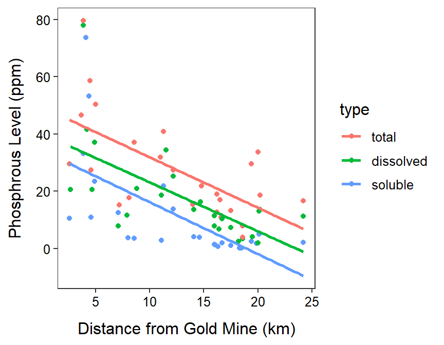
The ultimate full model is \(\mu_{P|DIST,\cdots} = \alpha+\beta DIST+\)\(\delta_{1}DP+\delta_{2}SP+\) \(\gamma_{1}DIST:DP+\gamma_{2}DIST:SP\) wher \(P\) is the phosphorous level, \(DIST\) is the distance from the gold mine, and the other variables were defined on the previous assignment.
Table shown below

Type	DP	SP	Sub-Model (\(\mu_{P\|DIST}=\))
Total P	0	0	\(\alpha+\beta DIST\)
Total Dissolved P	1	0	\((\alpha+\delta_{1})+(\beta+\gamma_{1})DIST\)
Soluble Reactive P	0	1	\((\alpha+\delta_{2})+(\beta+\gamma_{2})DIST\)

The “covariate” (distance) estimate is \(\hat{\beta}\) and thus means that the mean total (reference group) phosphorous level will decrease by 1.76 ppm when the distance from the gold mine increases by 1 km.
The “(Intercept)” estimate is \(\hat{\alpha}\) and thus means that the mean total (reference group) phosphorous at 0 km from the gold mine is 49.52 ppm.
The first indicator (typedissolved) estimate is \(\hat{\delta}_{1}\) and thus means that the y-intercept for dissolve phosphorous is 9.31 ppm less than the y-intercept for total phosphorous. The, the mean dissolved phosphorous is lower than the mean total phosphorous 0 km from the gold mine.
The second interaction (distance:typesoluble) estimate is \(\hat{\gamma}_{2}\) and thus means that the slope for solube phosphorous is 0.05 less than the slope for total phosphorous. Thus, solube phosphorous declines at a slower rate than total phosphrous as you move away from the gold mine.
The figure is below.

R Code and Results

gm <- read.csv("http://derekogle.com/NCMTH207/modules/ce/data/GoldMine.csv")
gm$type <- factor(gm$type,levels=c("total","dissolved","soluble"))
ivr.gm <- lm(phosp~distance+type+distance:type,data=gm)
cfs.gm <- cbind(Ests=coef(ivr.gm),confint(ivr.gm))
cbind(Est=coef(ivr.gm),confint(ivr.gm))

                                Est      2.5 %     97.5 %
(Intercept)             49.52108103  37.254998 61.7871642
distance                -1.76331862  -2.635300 -0.8913374
typedissolved           -9.31068754 -27.156010  8.5346350
typesoluble            -15.18830863 -32.560995  2.1843779
distance:typedissolved   0.05362709  -1.191473  1.2987269
distance:typesoluble    -0.04993832  -1.287360  1.1874829

ggplot(data=gm,mapping=aes(x=distance,y=phosp,color=type)) +  
  geom_point() +  
  labs(x="Distance from Gold Mine (km)",y="Phosphrous Level (ppm)") +  
  theme_NCStats() +  
  geom_smooth(method="lm",se=FALSE)

`geom_smooth()` using formula 'y ~ x'