Turtle Nesting Ecology
Note:
- When checking assumptions don’t say the residual plot looks normal unless it really does. The assumption is adequately met if the histogram is “not strongly skewed” which was the case here.
- For questions 6-8, you need to explicitly say that you are looking at the mean clutch size AT THE MEAN CARAPACE LENGHT (or maximum for #8) … don’t just say intercept as the question was specific. Also, these questions are asking you to interpret the DIFFERENCE, so you use the results from CONTRASTS portion of the output. The results in the EMMEANS portion of the output is about the mean clutch size for each group, not the differences among pairs of groups.
- When deciding what is most and least different, use the estimated difference not the p-value. The p-value is affected by sample size and variabiity, whereas the estimated difference measures just that.
- The turtles appear to be independent as there is no clear connection between individual turtles either within or among the regions. Turtles within a region could be familially connected but there is no indication that this happened. Of course, one could argue a connection within regions but that is the factor being explored so any dependencies there should be revealed in the analysis.
The residual plot show no curvature or obvious funneling, so the linearity and homoscedasticity assumptions appear to be met. The histogram of residuals is apparently not normal (Anderson-Darling p=0.0292) but is is not strongly skewed to the normality assumption is adequately met. There are two potential outliers evident in the lower-right corner of the residual plot and the left tail of the histogram of residuals but these are not statistically significant (outlier test p=0.0521). Thus, the assumptions are adequately met on the original scale and no transformation is needed. - No transformation is needed, the assumptions are adequately met.
- No need to identify which group slopes are different because the parallel lines test indicates that no slopes differ (p=0.1192).
- Not needed as no slopes differ.
- It is appropriate to check for differences in intercepts because the coincident lines test indicates that some intercepts do differ (p<0.00005). It appears that the intercept for the Arabian Gulf differs from the intercept of Red Sea, Caribbean, and West Atlantic regions (0.0026), but not from the Indian Ocean (p=0.0906). None of the intercepts from the Indian Ocean, Red Sea, Caribbean, and West Atlantic regions differ (0.7315).
- The mean clutch size at the mean curved carapace length is between 12.08 and 49.80 lower for turtles from the Arabian Gulf than those from the West Atlantic.
- The mean clutch size at the mean curved carapace length is between 14.89 lower and 8.61 greater for turtles from the Caribbean than those from the West Atlantic.
- The mean clutch size at the maximum curved carapace length does NOT differ between turtles from the Indian Ocean and West Atlantic regions (p=0.7315). Because the lines for these two regions are parallel evidence for a significant difference at any one curved carapace length (i.e., along the x-axis) is evidence for a significant difference at all curved carapace lengths. Of course, the opposite (not a significant difference) holds true as well.
R Code and Results
ht <- read.csv("https://raw.githubusercontent.com/droglenc/NCData/master/HawksbillTurtles.csv")
ht$Region <- factor(ht$Region,
                    levels=c("Arabian Gulf","Indian Ocean","Red Sea",
                             "Caribbean","West Atlantic"))
ivr.ht <- lm(Clutch.Size~CCL+Region+CCL:Region,data=ht)
anova(ivr.ht)
Analysis of Variance Table
Response: Clutch.Size
Df Sum Sq Mean Sq F value Pr(>F)
CCL 1 246757 246757 526.8775 < 2.2e-16
Region 4 22045 5511 11.7675 5.266e-09
CCL:Region 4 3461 865 1.8472 0.1192
Residuals 368 172349 468 assumptionCheck(ivr.ht)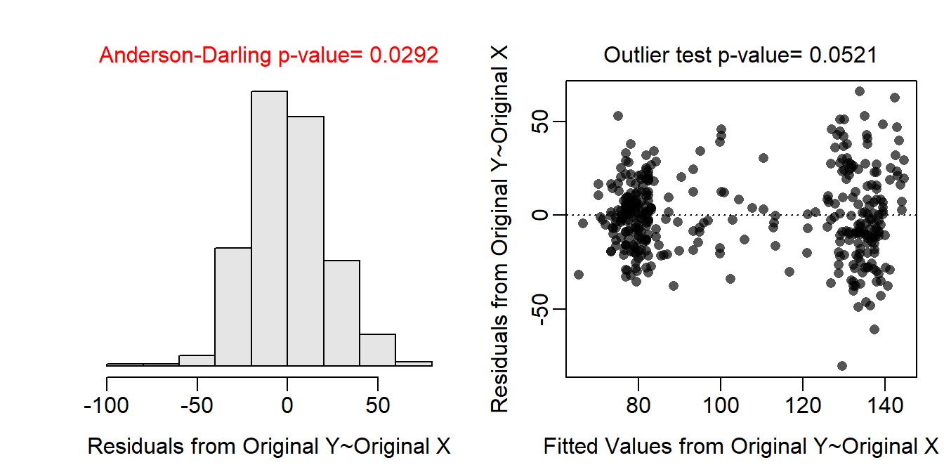
ivr.ht2 <- lm(Clutch.Size~CCL+Region,data=ht)
ivr.mc2 <- emmeans(ivr.ht2,pairwise~Region)
( ivr.mcsum2 <- summary(ivr.mc2,infer=TRUE) )
$emmeans
Region emmean SE df lower.CL upper.CL t.ratio p.value
Arabian Gulf 90.6 3.31 372 84.1 97.1 27.406 <.0001
Indian Ocean 109.2 7.87 372 93.8 124.7 13.880 <.0001
Red Sea 112.6 5.36 372 102.0 123.1 20.985 <.0001
Caribbean 118.4 4.68 372 109.2 127.6 25.277 <.0001
West Atlantic 121.5 4.50 372 112.7 130.4 26.999 <.0001
Confidence level used: 0.95
$contrasts
contrast estimate SE df lower.CL upper.CL t.ratio p.value
Arabian Gulf - Indian Ocean -18.64 7.43 372 -39.0 1.72 -2.510 0.0906
Arabian Gulf - Red Sea -21.97 4.57 372 -34.5 -9.43 -4.802 <.0001
Arabian Gulf - Caribbean -27.80 7.58 372 -48.6 -7.03 -3.668 0.0026
Arabian Gulf - West Atlantic -30.94 6.88 372 -49.8 -12.08 -4.497 0.0001
Indian Ocean - Red Sea -3.33 8.41 372 -26.4 19.73 -0.396 0.9948
Indian Ocean - Caribbean -9.16 10.49 372 -37.9 19.59 -0.873 0.9065
Indian Ocean - West Atlantic -12.30 9.97 372 -39.6 15.03 -1.234 0.7315
Red Sea - Caribbean -5.84 8.86 372 -30.1 18.44 -0.659 0.9649
Red Sea - West Atlantic -8.98 8.20 372 -31.5 13.51 -1.094 0.8094
Caribbean - West Atlantic -3.14 4.29 372 -14.9 8.61 -0.732 0.9489
Confidence level used: 0.95
Conf-level adjustment: tukey method for comparing a family of 5 estimates
P value adjustment: tukey method for comparing a family of 5 estimates
Water Quality Near a Gold Mine
- The phosphorous measurements do not appear to be independent either within or among types. First, there is a clear lack of independence among types as each type was recorded at the same location – of phosphorous level is high for one type at a location it is likely higher for the other types. There is a lack of independence within groups because the measurements are arranged spatially (distance from the goldmine). Both of these issues, however, are related to the explanatory variables in the analysis so it is likely OK to proceed.
The residual plot shows a clear curvature and obvious funneling, so the linearity and homoscedasticity assumptions are not met. The histogram of residuals is apparently not normal (Anderson-Darling p=0.0003) and is fairly strongly right-skewed so the normality assumption is not met. There are clear outliers (outlier test p=0.0192). Thus, the assumptions are not met on the original scale so a transformation is needed. - Log-transforming the phosphorous level results in a residual plot that does not exhibit curvature or funneling; thus, the linearity and homoscedasticity assumptions are met on this scale. The histogram of residuals is normal (Anderson-Darling p=0.6218) and is not strongly skewed so the normality assumption is adequately met. There are no outliers evident (outlier test p=0.5530). Thus, the assumptions are adequately met on the log-transformed phosphorous level scale.
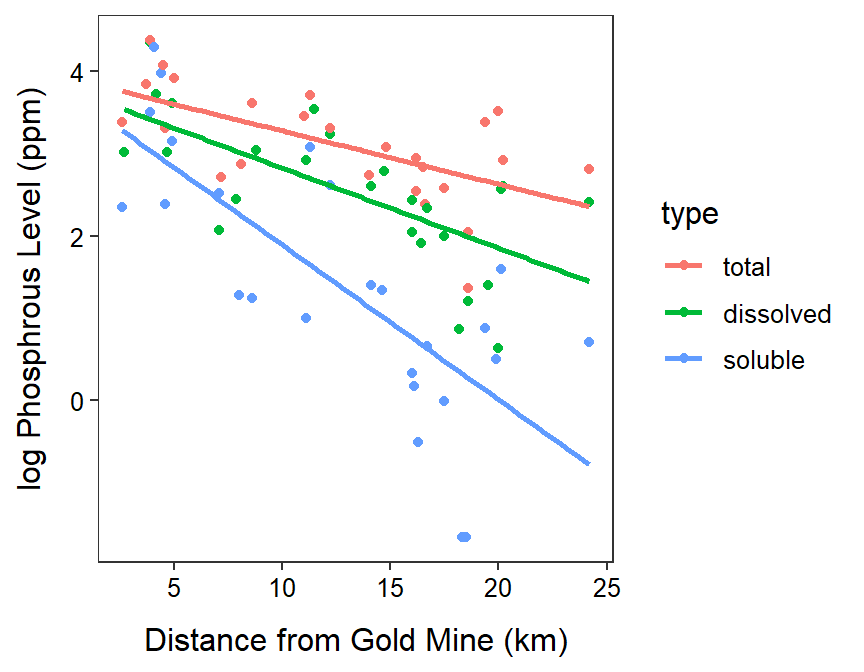
- The parallel lines test indicates that the slopes differ between some types of phosphorous (p=0.0029). In fact it appears that the slope for the soluble phosphorous is less than the slope for both total (p=0.0001) and dissolved (p=0.0012) phosphorous. There was no difference in slopes between total and dissolved phosphorous (p=0.3937).
- The slope for total phosphorous is between 1.056 and 1.198 greater than the slope for soluble phosphorous.
- The slope for total phosphorous is between 0.986 lower and 1.050 greater than the slope for dissolved phosphorous.
- The slope for the total phosphorous type indicates that as the distance from the gold mine increases by 1 km that mean total phosphorus declines by a multiple between 0.963 and 0.996.
- It is not appropriate to discuss differences in intercepts because the lines are not parallel.
- It is not appropriate to discuss differences in intercepts because the lines are not parallel.
R Code and Results
gm <- read.csv("http://derekogle.com/NCMTH207/modules/ce/data/GoldMine.csv")
gm$type <- factor(gm$type,levels=c("total","dissolved","soluble"))
ivr.gm <- lm(phosp~distance+type+distance:type,data=gm)
assumptionCheck(ivr.gm)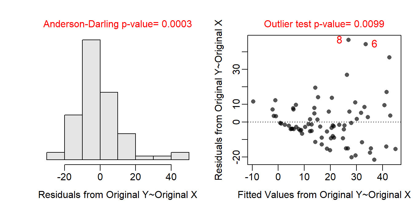
assumptionCheck(ivr.gm,lambday=0)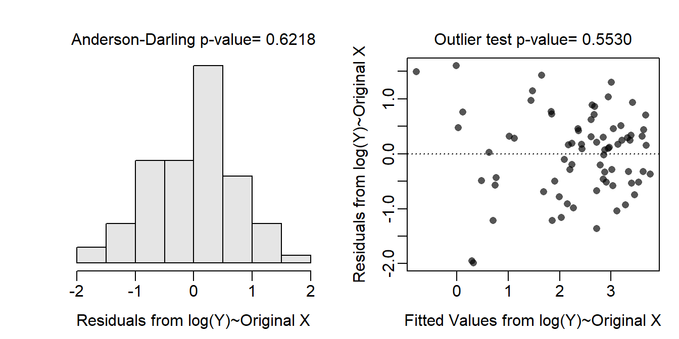
gm$logphosp <- log(gm$phosp)
ivr.gmt <- lm(logphosp~distance+type+distance:type,data=gm)
mc.gmt <- emtrends(ivr.gmt,specs=pairwise~type,var="distance",tran="log")
( mcsum.gmt <- summary(mc.gmt,infer=TRUE,type="response") )
$emtrends
type response SE df lower.CL upper.CL null t.ratio p.value
total 0.979 0.00809 69 0.963 0.996 1 -2.538 0.0134
dissolved 0.963 0.00981 69 0.943 0.982 1 -3.745 0.0004
soluble 0.871 0.02182 69 0.828 0.915 1 -5.525 <.0001
Confidence level used: 0.95
Intervals are back-transformed from the log scale
Tests are performed on the log scale
$contrasts
contrast ratio SE df lower.CL upper.CL null t.ratio p.value
total / dissolved 1.02 0.0133 69 0.986 1.05 1 1.311 0.3937
total / soluble 1.12 0.0297 69 1.056 1.20 1 4.453 0.0001
dissolved / soluble 1.11 0.0299 69 1.036 1.18 1 3.707 0.0012
Confidence level used: 0.95
Conf-level adjustment: tukey method for comparing a family of 3 estimates
Intervals are back-transformed from the log scale
P value adjustment: tukey method for comparing a family of 3 estimates
Tests are performed on the log scale ggplot(data=gm,mapping=aes(x=distance,y=logphosp,color=type)) +
geom_point() +
labs(x="Distance from Gold Mine (km)",y="log Phosphrous Level (ppm)") +
theme_NCStats() +
geom_smooth(method="lm",se=FALSE)`geom_smooth()` using formula 'y ~ x'