- Refer to specific p-values and graphs when demonstrating that the assumptions are met.
- Use the ANOVA table p-value when testing for a difference in group means.
- In question 2 be careful to state that it is the mean of the transformed variable that differs (not the mean of the untransformed variable).
- Use Tukey’s multiple comparison results when identifying specifically which pairs of group means differ.
- In questions 3-5 you must specifically refer to the mean of the transformed variable.
- Note that when the square root transformation was used that the group mean could be back-transformed (question 6) but the difference in group means could not (question 7).
- Note that when the log transformation was used that both the group mean (question 6) and the difference in group means (question 7) could be back-transformed.
- I find it hard to interpret the back-transformed difference in means (from the log scale) when the ratio is less than 1. Thus, I prefer to flip the ratio and talk about how the second group is that many times larger than the first group.
Assumptions I
- After square root transforming, the variances appear to be equal as suggested by the Levene’s test (p=0.2518) and the similar sized boxes in the boxplots below. The residuals appear to be normally distributed according to the Anderson-Darling test (p=0.2174) and the histogram below does not look strongly skewed. There is no evidence for a significant outlier according to the outlier test (p=0.2832).
- There appears to be a difference in mean square root of the measurement variable among some of the group means (ANOVA p<0.00005).
- It appears that mean square root of the measurement variable differs between all pairs of groups (p<0.00005), except for the “B” and “D” groups (p=0.8013).
- The mean square root of the measurement variable for the “A” group is between 8.48 and 11.36.
- The mean square root of the measurement variable is betwen 6.439 and 11.794 units less for the “A” group than for the “B” group.
- The back-transformed mean of the measurement variable for the “A” group is between 71.97 (=8.482) and 128.94 (=11.362).
- The differences in square root transformed values can not be back-transformed!
R Code and Results.
> df1 <- read.csv("http://derekogle.com/NCMTH207/modules/ce/data/ANOVA1Assumptions1.csv")
> lm1 <- lm(measure~group,data=df1)
> assumptionCheck(lm1,lambday=0.5)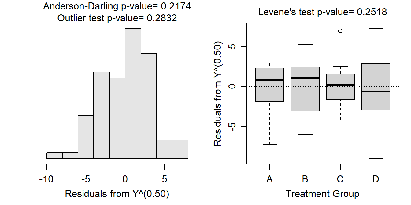
> df1$sqrtmeas <- sqrt(df1$measure)
> lm1t <- lm(sqrtmeas~group,data=df1)
> anova(lm1t)
Analysis of Variance Table
Response: sqrtmeas
Df Sum Sq Mean Sq F value Pr(>F)
group 3 3610.9 1203.62 115.82 < 2.2e-16
Residuals 76 789.8 10.39 > mc1t <- emmeans(lm1t,specs=pairwise~group,tran="sqrt")Note: Use 'contrast(regrid(object), ...)' to obtain contrasts of back-transformed estimates> ( mcsum1t <- summary(mc1t,infer=TRUE) )$emmeans
group emmean SE df lower.CL upper.CL t.ratio p.value
A 9.92 0.721 76 8.48 11.4 13.761 <.0001
B 19.04 0.721 76 17.60 20.5 26.408 <.0001
C 28.90 0.721 76 27.46 30.3 40.090 <.0001
D 19.96 0.721 76 18.52 21.4 27.690 <.0001
Results are given on the sqrt (not the response) scale.
Confidence level used: 0.95
$contrasts
contrast estimate SE df lower.CL upper.CL t.ratio p.value
A - B -9.117 1.02 76 -11.79 -6.44 -8.943 <.0001
A - C -18.979 1.02 76 -21.66 -16.30 -18.618 <.0001
A - D -10.041 1.02 76 -12.72 -7.36 -9.849 <.0001
B - C -9.863 1.02 76 -12.54 -7.18 -9.675 <.0001
B - D -0.924 1.02 76 -3.60 1.75 -0.907 0.8013
C - D 8.939 1.02 76 6.26 11.62 8.768 <.0001
Note: contrasts are still on the sqrt scale
Confidence level used: 0.95
Conf-level adjustment: tukey method for comparing a family of 4 estimates
P value adjustment: tukey method for comparing a family of 4 estimates > ( mcsum1bt <- summary(mc1t,infer=TRUE,type="response") )$emmeans
group response SE df lower.CL upper.CL t.ratio p.value
A 98.4 14.3 76 72 129 13.761 <.0001
B 362.4 27.4 76 310 419 26.408 <.0001
C 835.1 41.7 76 754 920 40.090 <.0001
D 398.4 28.8 76 343 458 27.690 <.0001
Confidence level used: 0.95
Intervals are back-transformed from the sqrt scale
Tests are performed on the sqrt scale
$contrasts
contrast estimate SE df lower.CL upper.CL t.ratio p.value
A - B -9.117 1.02 76 -11.79 -6.44 -8.943 <.0001
A - C -18.979 1.02 76 -21.66 -16.30 -18.618 <.0001
A - D -10.041 1.02 76 -12.72 -7.36 -9.849 <.0001
B - C -9.863 1.02 76 -12.54 -7.18 -9.675 <.0001
B - D -0.924 1.02 76 -3.60 1.75 -0.907 0.8013
C - D 8.939 1.02 76 6.26 11.62 8.768 <.0001
Note: contrasts are still on the sqrt scale
Confidence level used: 0.95
Conf-level adjustment: tukey method for comparing a family of 4 estimates
P value adjustment: tukey method for comparing a family of 4 estimates
Assumptions II
- After log transforming, the variances appear to be equal as suggested by the Levene’s test (p=0.7675) and the similar sized boxes in the boxplots below. The residuals appear to be normally distributed according to the Anderson-Darling test (p=0.5422) and the histogram below does not look strongly skewed. There is no evidence for a significant outlier according to the outlier test (p=0.9257).
- There appears to be a difference in mean log of the measurement variable among some of the group means (ANOVA p<0.00005).
- It appears that mean log of the measurement variable differs between all three groups (p<0.0135).
- The mean log of the measurement variable for the “A” group is between 1.81 and 2.56.
- The mean log of the measurement variable is between 0.135 and 1.415 units greater for the “A” group than for the “B” group.
- The back-transformed mean of the measurement variable for the “A” group is between 6.08 (=e1.81) and 12.94 (=e2.56).
- The back-transformed mean of the measurement variable for the “A” group is between 1.144 and 4.114 TIMES larger than the back-transformed mean for the “B” group.
R Code and Results.
> df2 <- read.csv("http://derekogle.com/NCMTH207/modules/ce/data/ANOVA1Assumptions2.csv")
> lm2 <- lm(measure~group,data=df2)
> assumptionCheck(lm2,lambday=0)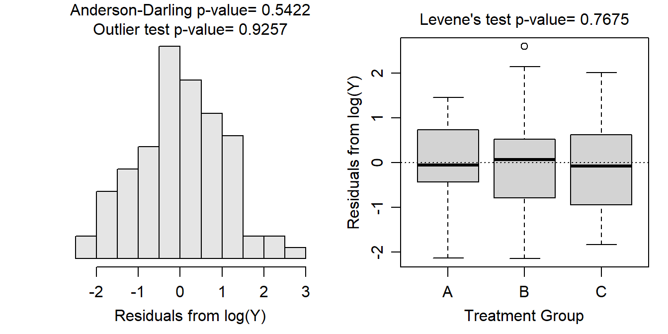
> df2$logmeas <- log(df2$measure)
> lm2t <- lm(logmeas~group,data=df2)
> anova(lm2t)
Analysis of Variance Table
Response: logmeas
Df Sum Sq Mean Sq F value Pr(>F)
group 2 46.417 23.2085 21.484 2.613e-08
Residuals 87 93.983 1.0803 > mc2t <- emmeans(lm2t,specs=pairwise~group,tran="log")
> ( mcsum2t <- summary(mc2t,infer=TRUE) )$emmeans
group emmean SE df lower.CL upper.CL t.ratio p.value
A 2.18 0.19 87 1.81 2.56 11.504 <.0001
B 1.41 0.19 87 1.03 1.79 7.422 <.0001
C 3.16 0.19 87 2.79 3.54 16.671 <.0001
Results are given on the log (not the response) scale.
Confidence level used: 0.95
$contrasts
contrast estimate SE df lower.CL upper.CL t.ratio p.value
A - B 0.775 0.268 87 0.135 1.415 2.886 0.0135
A - C -0.980 0.268 87 -1.620 -0.341 -3.654 0.0013
B - C -1.755 0.268 87 -2.395 -1.115 -6.540 <.0001
Results are given on the log (not the response) scale.
Confidence level used: 0.95
Conf-level adjustment: tukey method for comparing a family of 3 estimates
P value adjustment: tukey method for comparing a family of 3 estimates > ( mcsum2bt <- summary(mc2t,infer=TRUE,type="response") )$emmeans
group response SE df lower.CL upper.CL null t.ratio p.value
A 8.87 1.684 87 6.08 12.94 1 11.504 <.0001
B 4.09 0.776 87 2.80 5.96 1 7.422 <.0001
C 23.65 4.488 87 16.22 34.49 1 16.671 <.0001
Confidence level used: 0.95
Intervals are back-transformed from the log scale
Tests are performed on the log scale
$contrasts
contrast ratio SE df lower.CL upper.CL null t.ratio p.value
A / B 2.170 0.5823 87 1.1442 4.114 1 2.886 0.0135
A / C 0.375 0.1007 87 0.1978 0.711 1 -3.654 0.0013
B / C 0.173 0.0464 87 0.0912 0.328 1 -6.540 <.0001
Confidence level used: 0.95
Conf-level adjustment: tukey method for comparing a family of 3 estimates
Intervals are back-transformed from the log scale
P value adjustment: tukey method for comparing a family of 3 estimates
Tests are performed on the log scale
Iron and Mining
- After log transforming, the variances appear to be equal as suggested by the Levene’s test (p=0.4719) and the similarity in the boxes in the boxplot below. The Anderson-Darling test suggests that the residuals are not normally distributed (p=0.0004), but the histogram below is not strongly skewed so this assumption is adequately met. There is no strong evidence for a significant outlier according to the outlier test (p=0.0565).
- There appears to be a difference in mean log iron concentration in streams among some of the basin types (ANOVA p<0.00005).
- It appears that mean log iron concentration in mines in basins with abandoned mines differs from basins with reclaimed mines (p<0.00005) and basins that were unmined (p<0.00005). The mean log concentration did not differ between streams in basins with reclaimed mines and basins that were not mined (p=0.0694).
- The mean log concentration of iron was lowest in streams in the unmined basin at between -1.748 and -0.823.
- The back-transformed mean concentration of iron in streams in the unmined basin is between 0.174 mg/L (=e-1.748) and 0.439 mg/L (=e-0.823).
- The mean log concentration of iron in streams in the unmined basin was between 1.392 and 3.006 units less than the mean log concentration of iron in streams in basins with abandoned mines.
- The mean concentration of iron in streams in the unmined basin was between 0.050 and 0.248 as large as the mean concentration of iron in streams in the basin with abandoned mines. Alternatively, mean concentration of iron in streams in the basin with abandoned mines was between 4.024 and 20.198 times larger than the mean concentration of iron in streams in the unmined basin.
R Code and Results.
> im <- read.csv("https://raw.githubusercontent.com/droglenc/NCData/master/AcidMineDrainage.csv")
> im$use <- factor(im$use,levels=c("Unmined","Reclaimed","Abandoned"))
> lm3 <- lm(FE~use,data=im)
> assumptionCheck(lm3,lambday=0)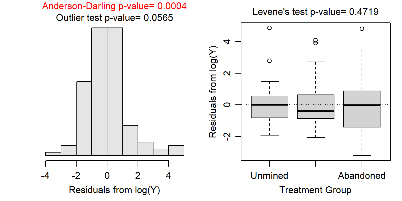
> im$logFE <- log(im$FE)
> lm3t <- lm(logFE~use,data=im)
> anova(lm3t)
Analysis of Variance Table
Response: logFE
Df Sum Sq Mean Sq F value Pr(>F)
use 2 90.091 45.045 21.743 9.35e-09
Residuals 117 242.392 2.072 > mc3t <- emmeans(lm3t,specs=pairwise~use,tran="log")
> ( mcsum3t <- summary(mc3t,infer=TRUE) )$emmeans
use emmean SE df lower.CL upper.CL t.ratio p.value
Unmined -1.286 0.233 117 -1.748 -0.823 -5.506 <.0001
Reclaimed -0.587 0.208 117 -0.998 -0.175 -2.825 0.0056
Abandoned 0.913 0.247 117 0.425 1.402 3.700 0.0003
Results are given on the log (not the response) scale.
Confidence level used: 0.95
$contrasts
contrast estimate SE df lower.CL upper.CL t.ratio p.value
Unmined - Reclaimed -0.699 0.313 117 -1.44 0.0432 -2.236 0.0694
Unmined - Abandoned -2.199 0.340 117 -3.01 -1.3923 -6.472 <.0001
Reclaimed - Abandoned -1.500 0.323 117 -2.27 -0.7343 -4.650 <.0001
Results are given on the log (not the response) scale.
Confidence level used: 0.95
Conf-level adjustment: tukey method for comparing a family of 3 estimates
P value adjustment: tukey method for comparing a family of 3 estimates > ( mcsum3bt <- summary(mc3t,infer=TRUE,type="response") )$emmeans
use response SE df lower.CL upper.CL null t.ratio p.value
Unmined 0.276 0.0646 117 0.174 0.439 1 -5.506 <.0001
Reclaimed 0.556 0.1155 117 0.369 0.839 1 -2.825 0.0056
Abandoned 2.493 0.6153 117 1.529 4.064 1 3.700 0.0003
Confidence level used: 0.95
Intervals are back-transformed from the log scale
Tests are performed on the log scale
$contrasts
contrast ratio SE df lower.CL upper.CL null t.ratio p.value
Unmined / Reclaimed 0.497 0.1554 117 0.2368 1.044 1 -2.236 0.0694
Unmined / Abandoned 0.111 0.0377 117 0.0495 0.248 1 -6.472 <.0001
Reclaimed / Abandoned 0.223 0.0720 117 0.1037 0.480 1 -4.650 <.0001
Confidence level used: 0.95
Conf-level adjustment: tukey method for comparing a family of 3 estimates
Intervals are back-transformed from the log scale
P value adjustment: tukey method for comparing a family of 3 estimates
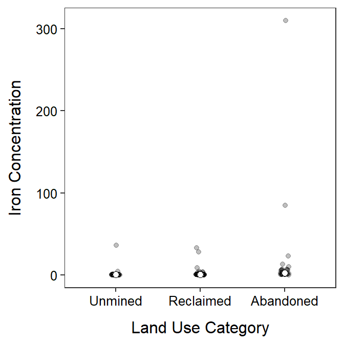
Tests are performed on the log scale > p1 <- ggplot() +
geom_jitter(data=im,mapping=aes(x=use,y=FE),alpha=0.25,width=0.05) +
geom_errorbar(data=mcsum3bt$emmeans,
mapping=aes(x=use,y=response,ymin=lower.CL,ymax=upper.CL),
size=2,width=0) +
geom_point(data=mcsum3bt$emmeans,mapping=aes(x=use,y=response),
size=2,pch=21,fill="white") +
labs(y="Iron Concentration",x="Land Use Category") +
theme_NCStats()
> p1
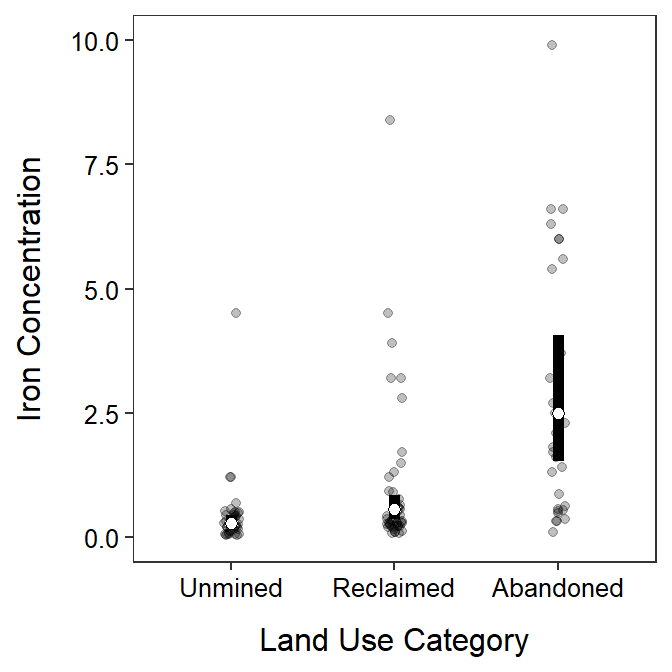
> p1 +
coord_cartesian(ylim=c(0,10))