- Refer to specific p-values and graphs when demonstrating that the assumptions are met.
- Refer to specific p-values for all tests.
- Use the ANOVA table p-value when testing for a difference in group means. Make sure when interpreting the ANOVA p-value that your language does not make it sound like all means differ … you don’t know that yet.
Speed and Distance Estimation
The statistical hypotheses to be examined are
\[ \begin{split} H_{0}&: \mu_{Non-Practitioner} = \mu_{Individual} = \mu_{Team Sport} \\ H_{A}&:\text{At least one pair of means is different} \end{split} \]
where μ is the mean “score” on the speed and distance estimation tests and the subscripts identify the different types of participation in sports.
The study is balanced as there are the same number of individuals in each participation group. The sample size (=32) seems adequate.
The individuals are likely independent but there are some issues to consider. Within the sports participation groups there are some individuals that came from the same team or club. These individuals may be related in some way; e.g., perhaps the team is “elite” such that you would expect the individuals to be excellent at these tests. However, not all individuals are from the same team or club so this is likely not a barrier to independence. There does not seem to be any relationships between individuals across the sports participation groups – i.e., individuals in the different groups don’t appear to be familially related, etc. The data are likely independent enough for our purposes.
The residuals appear normal (Anderson-Darling p=0.0628) and the histogram below is only slightly skewed, the variances appear equal (Levene’s p=0.5308), and there are no significant outliers (outlier test p<0.00005). Thus, the assumptions are met on the original scale and no transformation will be considered.
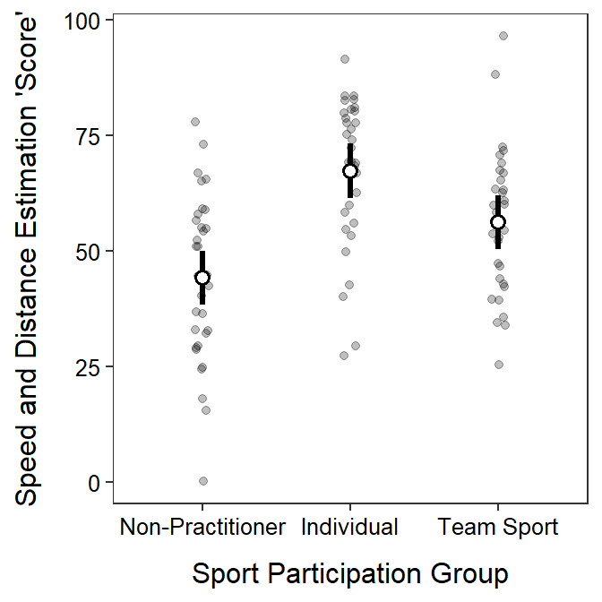
There appears to be a difference in mean speed and distance estimation “score” among some of the sports participation groups (ANOVA p<0.00005). In fact it appears that all three groups differ from each other (Tukey p≤0.0243). Specifically, mean speed and distance estimation “score” for non-practitioners was lower than that for the other two groups – between 13.21 and 33.09 lower than for those participating in individual sports and between 2.082 and 21.96 lower than for those participating in team sports. Additionally, those participating in individuals sports had mean speed and distance estimation “scores” between 1.191 and 21.07 higher than that for those participating in team sports.
These results indicate that those that participate in sports have higher speed and distance estimation scores than those that do not participated in sports. Furthermore, participating in an individual sport than a team sports appears to be related to a higher speed and distance estimation score.
R Code and Results
> df <- read.csv("http://derekogle.com/NCMTH207/modules/ce/data/SDE.csv")
> df$Group <- factor(df$Group,levels=c("Non-Practitioner","Individual","Team Sport"))
> xtabs(~Group,data=df)
Group
Non-Practitioner Individual Team Sport
32 32 32 > lm2 <- lm(SDE~Group,data=df)
> assumptionCheck(lm2)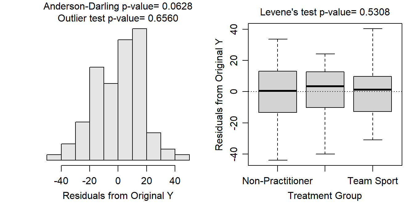
> anova(lm2)Analysis of Variance Table
Response: SDE
Df Sum Sq Mean Sq F value Pr(>F)
Group 2 8581.2 4290.6 15.397 1.675e-06
Residuals 93 25916.3 278.7 > mc2 <- emmeans(lm2,specs=pairwise~Group)
> ( mcsum2 <- summary(mc2,infer=TRUE) )$emmeans
Group emmean SE df lower.CL upper.CL t.ratio p.value
Non-Practitioner 44.1 2.95 93 38.2 50.0 14.941 <.0001
Individual 67.2 2.95 93 61.4 73.1 22.787 <.0001
Team Sport 56.1 2.95 93 50.3 62.0 19.015 <.0001
Confidence level used: 0.95
$contrasts
contrast estimate SE df lower.CL upper.CL t.ratio p.value
(Non-Practitioner) - Individual -23.2 4.17 93 -33.09 -13.21 -5.548 <.0001
(Non-Practitioner) - Team Sport -12.0 4.17 93 -21.96 -2.08 -2.881 0.0135
Individual - Team Sport 11.1 4.17 93 1.19 21.07 2.667 0.0243
Confidence level used: 0.95
Conf-level adjustment: tukey method for comparing a family of 3 estimates
P value adjustment: tukey method for comparing a family of 3 estimates > ggplot() +
geom_jitter(data=df,mapping=aes(x=Group,y=SDE),
alpha=0.25,width=0.05) +
geom_pointrange(data=mcsum2$emmeans,
mapping=aes(x=Group,y=emmean,ymin=lower.CL,ymax=upper.CL),
size=1.1,fatten=2,pch=21,fill="white") +
labs(x="Sport Participation Group",y="Speed and Distance Estimation 'Score'") +
theme_NCStats()