Raising Young Cuckoos

It is not appropriate to conduct multiple comparisons in this example because the H₀ in the one-way ANOVA was not rejected. This result suggests that there is no difference among group means and, thus, no need to determine which specific groups differ.

Temperature and Turtle Hatchings

On the first question, define any symbols used in the hypotheses.
On the second question, use the p-value from the ANOVA table. That is the p-value that assesses whether all group means are equal or not. Tukey’s multiple comparisons are only used to assess difference in paired means AFTER it has been determined that there is a difference in means.
On teh second and third questions, make sure to include the p-value (see below). The p-value is the evidence for your statement … don’t just make a statement without showing your evidence. Also, I would like to see the p-value in your sentence so it is clear to me what you are looking at … don’t just say “as seen below” (because there is lots of information below).
In the fourth question, clearly indicate which group is greater (or lesser). Don’t just say that you are 95% confident that the difference is between such-and-such.
In the fifth question include a plot of Tukey’s corrected means with confidence intervals.
In the last question, note that there is no difference in means for the first three temperatures. So, even though, the plot shows slight differences in the SAMPLE means, those differences were not great enough to conclude that the POPULATION means were different. So, your conclusion should not make it sound like there is a difference among those temperature treatments.
Also note in the fourth, fifth, and last questions that the conclusions are about the MEAN days to hatch not days to hatch because that is what is tested in the hypotheses. Make sure to include the word MEAN.
Note how concise the answer key is. Please work to get your answers this concise.

The H₀: μ_15C=μ_20C=μ_25C=μ_30C, where μ is the mean days to hatch and the subscripts are the temperatures in the temperature treatments. The H_A: “mean days to hatch differs between at least one pair of treatment temperatures”.
It appears that the mean days to hatch differs between at least one pair of treatment temperatures (p<0.00005<α).
It appears that the mean days to hatch differs between 30^oC and 15^oC (p<0.00005), 20^oC (p=0.0008), and 25^oC (p=0.0001). The mean days to hatch did not differ between any other pairs of temperature treatments (p>0.0983).
It appears that the mean days to hatch at 30^oC was between 22.7 and 53.9 days lower than at 15^oC, between 8.9 and 40.1 days lower than at 20^oC, and between 13.5 and 44.7 days lower than at 25^oC.
The plot of means with 95% confidence intervals is shown below.
It appears that temperature does not affect the mean days to hatch from between 15^oC to 25^oC, but declines dramatically from 25^oC to 30^oC. Thus, temperature does affect the mean days to hatch but not until temperature is above 25^oC.

R Code and Results.

> d <- read.csv("turtles.csv")
> d$Temperature <- factor(d$Temperature)

> lm1 <- lm(Days~Temperature,data=d)
> anova(lm1)

Analysis of Variance Table

Response: Days
            Df Sum Sq Mean Sq F value    Pr(>F)
Temperature  3 8025.5 2675.16  15.978 9.082e-07
Residuals   36 6027.3  167.42

> mc <- emmeans(lm1,specs=pairwise~Temperature)
> ( mcsum <- summary(mc,infer=TRUE) )

$emmeans
 Temperature emmean   SE df lower.CL upper.CL t.ratio p.value
 15            58.4 4.09 36     50.1     66.7  14.273  <.0001
 20            44.6 4.09 36     36.3     52.9  10.900  <.0001
 25            49.2 4.09 36     40.9     57.5  12.024  <.0001
 30            20.1 4.09 36     11.8     28.4   4.912  <.0001

Confidence level used: 0.95 

$contrasts
 contrast estimate   SE df lower.CL upper.CL t.ratio p.value
 15 - 20      13.8 5.79 36    -1.78     29.4   2.385  0.0983
 15 - 25       9.2 5.79 36    -6.38     24.8   1.590  0.3970
 15 - 30      38.3 5.79 36    22.72     53.9   6.619  <.0001
 20 - 25      -4.6 5.79 36   -20.18     11.0  -0.795  0.8563
 20 - 30      24.5 5.79 36     8.92     40.1   4.234  0.0008
 25 - 30      29.1 5.79 36    13.52     44.7   5.029  0.0001

Confidence level used: 0.95 
Conf-level adjustment: tukey method for comparing a family of 4 estimates 
P value adjustment: tukey method for comparing a family of 4 estimates

> ggplot(data=d,mapping=aes(x=Temperature,y=Days)) +
    geom_jitter(alpha=0.5,width=0.05) +
    geom_pointrange(data=mcsum$emmeans,
                    mapping=aes(x=Temperature,y=emmean,
                                ymin=lower.CL,ymax=upper.CL),
                 size=1.1,fatten=2,pch=21,fill="white") +
    labs(y="Days to Hatch",x="Temperature Treatment") +
    theme_NCStats()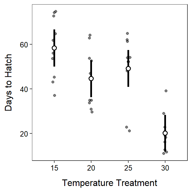

Salamander

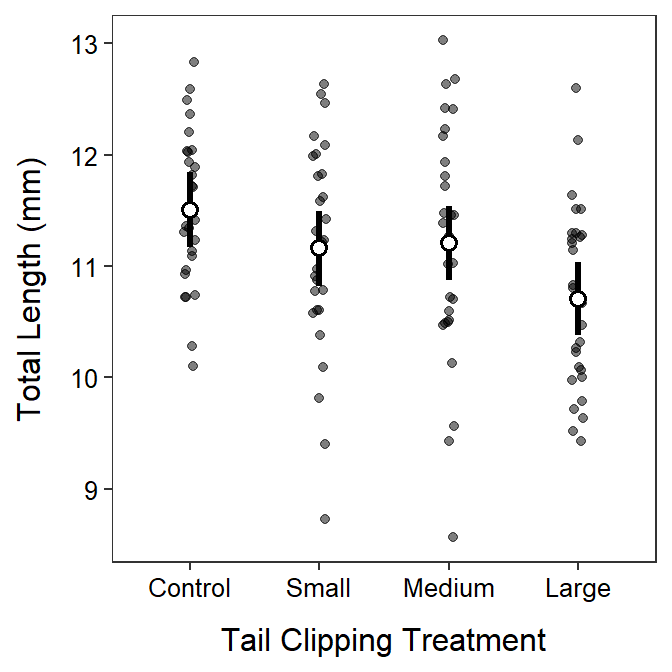
The H₀: μ_Control=μ_Small=μ_Medium=μ_Large, where μ is the mean total length at the end of the experiment and the subscripts are the tail clipping treatments. The H_A: “mean total length differs between at least one pair of tail clipping treatments”.
It appears that the total length differs between at least one pair of tail clipping treatments (p=0.0102<α).
It appears that the mean total length differs only between the control (no clipping) treatment and the “large” (10.0-mm) clipping treatment (p=0.0051). The mean total length did not differ between any other pairs of tail clipping treatments (p>0.1512).
It appears that the mean total length was between 0.2 and 1.4 mm lower in the “large” clipping treatment than the control (no clipping) treatment.
The plot of means with 95% confidence intervals is shown below.
It appears that clipping only results in a difference in mean total length if the large (10.0-mm) clipping is compared to no clipping (i.e., control). Part of the reason that few differences in mean total length were observed is because there is a large amount of natural variability among individuals in each group.

R Code and Results.

df <- read.csv("https://raw.githubusercontent.com/droglenc/NCData/master/Salamanders.csv")
df$Treatment <- factor(df$Treatment,levels=c("Control","Small","Medium","Large"))
lm2 <- lm(TL~Treatment,data=df)
anova(lm2)

Analysis of Variance Table

Response: TL
           Df Sum Sq Mean Sq F value  Pr(>F)
Treatment   3  9.348  3.1161   3.953 0.01017
Residuals 109 85.924  0.7883

mcS <- emmeans(lm2,specs=pairwise~Treatment)
( mcSsum <- summary(mcS,infer=TRUE) )

$emmeans
 Treatment emmean    SE  df lower.CL upper.CL t.ratio p.value
 Control     11.5 0.168 109     11.2     11.8  68.581  <.0001
 Small       11.2 0.168 109     10.8     11.5  66.495  <.0001
 Medium      11.2 0.168 109     10.9     11.5  66.793  <.0001
 Large       10.7 0.165 109     10.4     11.0  64.941  <.0001

Confidence level used: 0.95 

$contrasts
 contrast         estimate    SE  df lower.CL upper.CL t.ratio p.value
 Control - Small      0.35 0.237 109   -0.269    0.969   1.475  0.4561
 Control - Medium     0.30 0.237 109   -0.319    0.919   1.264  0.5875
 Control - Large      0.80 0.235 109    0.186    1.414   3.402  0.0051
 Small - Medium      -0.05 0.237 109   -0.669    0.569  -0.211  0.9967
 Small - Large        0.45 0.235 109   -0.164    1.064   1.914  0.2282
 Medium - Large       0.50 0.235 109   -0.114    1.114   2.127  0.1512

Confidence level used: 0.95 
Conf-level adjustment: tukey method for comparing a family of 4 estimates 
P value adjustment: tukey method for comparing a family of 4 estimates

ggplot(data=df,mapping=aes(x=Treatment,y=TL)) +
  geom_jitter(alpha=0.5,width=0.05) +
  geom_pointrange(data=mcSsum$emmeans,
                  mapping=aes(x=Treatment,y=emmean,ymin=lower.CL,ymax=upper.CL),
               size=1.1,fatten=2,pch=21,fill="white") +
  labs(y="Total Length (mm)",x="Tail Clipping Treatment") +
  theme_NCStats()