Growth of individual organisms within a population is generally characterized by an expression which is representative of individual growth of an “average” animal in the population. Individual growth is treated as an increase in either length or weight with increasing age. Several functions (or models) have been used to model the mean length or weight of fishes. One function, the von Bertalanffy growth function (VBGF), is the most popular and is the focus of this module.
Size-at-Age Data
The raw data for size-at-age modeling consists of the measurement of size, either length or weight, and the assignment of age to individual fish at the time the fish was captured. This is called length-at-capture, weight-at-capture, and age-at-capture data. An example1 of this type of data for length and age is shown in Table 1-Left and in Figure 1.
Table 1: Length-at-age for a portion of a sample of male Atlantic Croakers (left) and average length-at-age (right) for all male Atlantic Croakers in 1999.
| Individual Data | ||
|---|---|---|
| Indiv | Age | Length |
| 1 | 1 | 248 |
| 2 | 2 | 210 |
| 3 | 2 | 225 |
| 4 | 2 | 236 |
| 5 | 2 | 240 |
| 6 | 2 | 245 |
| 7 | 2 | 255 |
| 8 | 2 | 258 |
| 9 | 2 | 263 |
| 10 | 2 | 270 |
| 11 | 2 | 292 |
| \(\vdots\) | \(\vdots\) | \(\vdots\) |
| Summarized Data | |
|---|---|
| Avg Age | Avg Length |
| 1 | 248.0 |
| 2 | 248.4 |
| 3 | 281.8 |
| 4 | 298.3 |
| 5 | 328.2 |
| 6 | 345.9 |
| 7 | 332.5 |
| 8 | 344.3 |
| 9 | 370.8 |
| 10 | 327.0 |
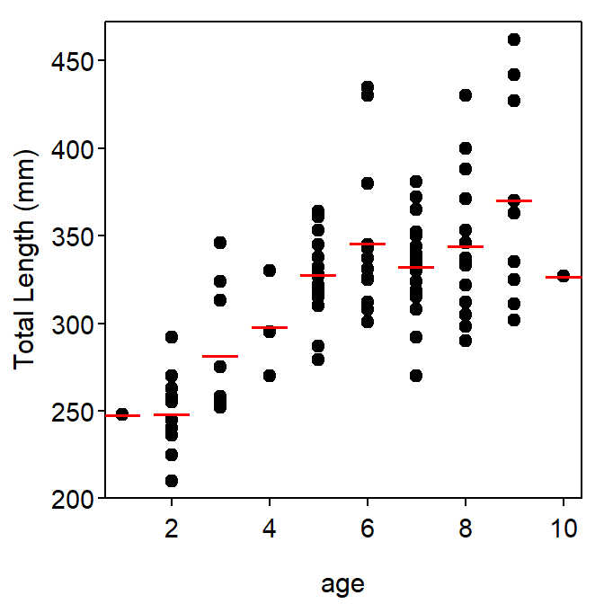
Figure 1: Length-at-age of male Atlantic Croaker. Red lines are the average length-at-age.
Historical methods for estimating the parameters of growth models used the average length or weight at each observed age for the sample (Table 1-Right) rather than the original data recorded for each individual. The historical methods should no longer be used because high-speed computers can easily perform the calculations or iterations necessary for fitting the growth models to individual at-capture data. In addition, the historical methods lost important information about individual variability. The historical method is carefully discussed in Ricker (1975).
It is also common to use “back-calculation” techniques to reconstruct data for growth analyses. This type of data is called retrospective size-at-age data (Jones 2000). Growth data generated in this way is generally inappropriate for the simple modeling techniques developed in this vignette because the back-calculated measurements are serially correlated (i.e., the techniques described here require independent observations). The problems created by serially-correlated data and techniques for handling serially-correlated data are described in Jones (2000).
“Typical” von Bertalanffy Growth Model
The Model and Parameters
There are many versions or parameterizations of the VBGF (see this section). The most common version is due to Beverton (1954) and Beverton and Holt (1957), who modified the original version introduced by von Bertalanffy (Cailliet et al. 2006). This model will be termed the “typical” version of the VBGF throughout this module. The typical VBGF is represented by2
\[ E[L|t] = L_{\infty}\left(1-e^{-K(t-t_{0})}\right) \quad \quad \text{(1)} \]
where
- \(E[L|t]\) is the expected or average length at time (or age) t,
- \(L_{\infty}\) is the asymptotic average length,
- \(K\) is the so-called Brody growth rate coefficient (units are yr\(^{-1}\)), and
- \(t_{0}\) is a modeling artificat that is said to represent the time or age when the average length was zero.
The parameters of Equation 1 have strict meanings that have been misunderstood in past work. The following items address some of these misunderstandings.
\(L_{\infty}\) is not the maximum length of the animal. Rather \(L_{\infty}\) is the asymptote for the model of average length-at-age (Francis 1988). As with any average, some individuals will be larger than average; thus, some animals will be larger than \(L_{\infty}\). This is illustrated in Figure 2.
Furthermore, Francis (1988) argues that \(L_{\infty}\) only has meaning in fish populations where “mortality is low enough to allow fish to reach an age at which the mean length (virtually) ceases to increase.”
\(K\) is not a growth rate (Ricker 1975). The units of \(K\) can be seen by algebraically solving Equation 1 for \(K\),
\[ 1-\frac{E[L|t]}{L_{\infty}} = -e^{-K(t-t_{o})} \] \[ log\left(\frac{1-E[L|t]}{L_{\infty}}\right) = -K(t-t_{o}) \] \[ K = \frac{log\left(\frac{L_{\infty}-E[L|t]}{L_{\infty}}\right)}{t-t_{o}} \]
- to notice that the units in the numerator disappear. Thus, the units of \(K\) are in \(time^{-1}\) rather than a change in length for a unit time as required by a growth rate.
- Schnute and Fournier (1980) offer two related interpretations of the meaning of \(K\). First, \(K\) “measures the exponential rate of approach to the asymptotic size.” Second, the value \(e^{-K}\) is “the fixed fraction by which the annual growth increment is multiplied each year.” This last definition is seen by the relation
\[ E[L|t=i+2]-E[L|t=i+1] = e^{-K}(E[L|t=i+1]-E[L|t=i]) \quad \quad \text{(2)} \]
- where, because \(K>0\), the quantity \(e^{-K}\) is a decimal. Thus, each succeeding growth increment is a constant fraction of the current growth increment indicating that growth slows as the fish gets older.
\(t_{0}\), despite its definition above, is a modeling artifact and not a biological parameter (Schnute and Fournier 1980). The \(t_{0}\) parameter is included in Equation 1 to adjust or “correct” the model for the initial size of the animal as most of the models do not pass through the origin. This is illustrated in Figure 2. Beverton (1954) said “It must be remembered that the constant \(t_{0}\) is largely artificial, insofar as it defines the age at which the organism would be of zero length if it grew throughout life with the same pattern of growth as in the post-larval stage.” In addition, Beverton and Holt (1957) stated that “in practice, the constant \(t_{0}\) must be regarded as quite artificial.”
The estimation and interpretation of \(t_{0}\) is further complicated by the fact that the value of \(t_{0}\) is generally an extrapolation (Francis 1988) – e.g., Figure 2.
\(L_{\infty}\), \(K\), and \(t_{0}\) are highly related (or correlated). This can be seen in the solution for \(K\) above where \(K\) depends on the values of \(L_{\infty}\) and \(t_{0}\). For example, with all else held constant, \(K\) will be larger for smaller values of \(L_{\infty}\). This dependency among parameters causes problems in model fitting and interpretation (Ratkowsky 1986). Some of the other VBGF parameterizations (see this section) have parameters that are much less correlated.
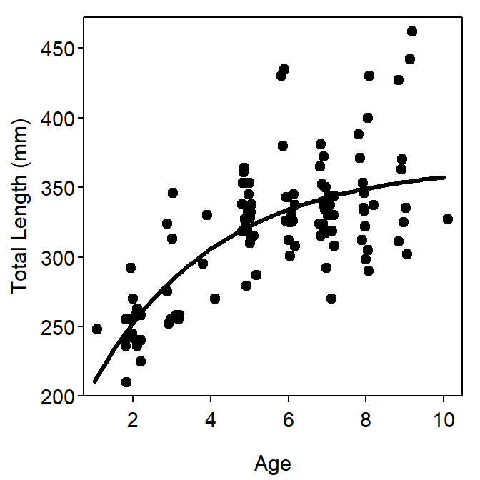
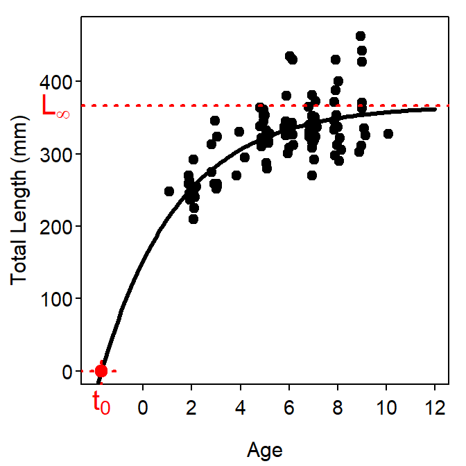
Figure 2: Example of the typical parameterization of the VBGF fit to size-at-age Atlantic Croaker data. The plot on the left is the fitted model expressed over the observed ages and lengths of the data. The plot on the right is the same fitted model but expressed over a range of ages and lengths that allow illustrating the meaning of \(L_{\infty}\) and \(t_{0}\).
Other Parameterizations of the VBGF
The Models and Their Parameters
A model can often be cast into a different parameterization where the model is functionally the same – i.e., predictions are exactly the same – but it has different parameters. Different parameterizations of models are created for a variety of reasons but two important reasons are that the re-parameterized model (i) has parameters for which the interpretation meets some need and (ii) has parameters that are less correlated. Each parameterization can ultimately be shown to be equivalent via albegra. The VBGF has been cast in at least five different parameterizations, each of which is discussed in this section.
Original Model Parameterization
The VBGF first proposed by von Bertalanffy (Cailliet et al. 2006) is
\[ E[L|t] = L_{\infty} - \left (L_{\infty} - L_{0}\right)e^{-Kt} \quad \quad \text{(3)} \]
where most items are defined as for Equation 1 and \(L_{0}\) is the mean length at time zero (i.e., birth).3 Visualizations for the parameters are shown in Figure 3. This parameterization of the VBGF, despite being the model proposed by von Bertalanffy, has been relatively (as compared to the typical VBGF) rarely used in the literature. However, Cailliet et al. (2006) recommended its use with chondrychthians.
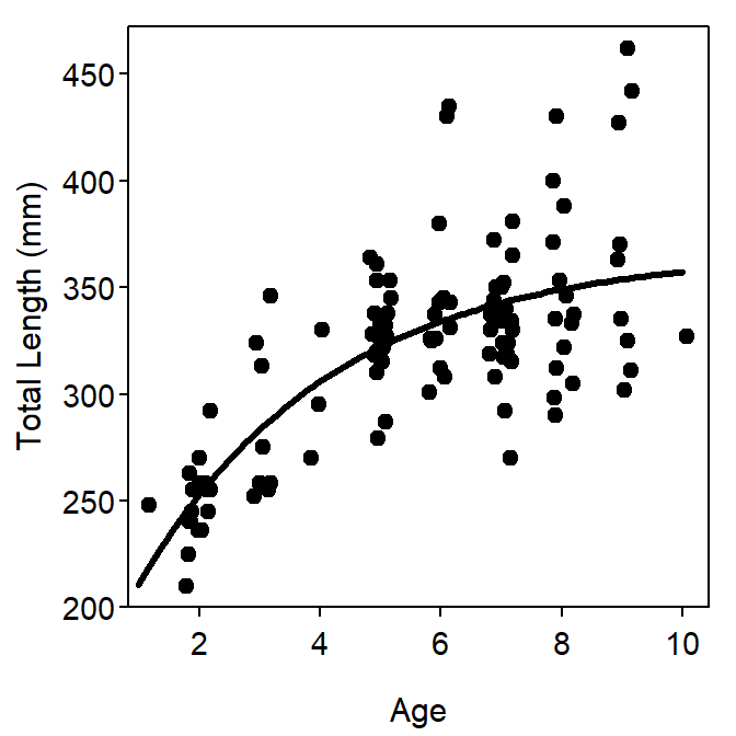
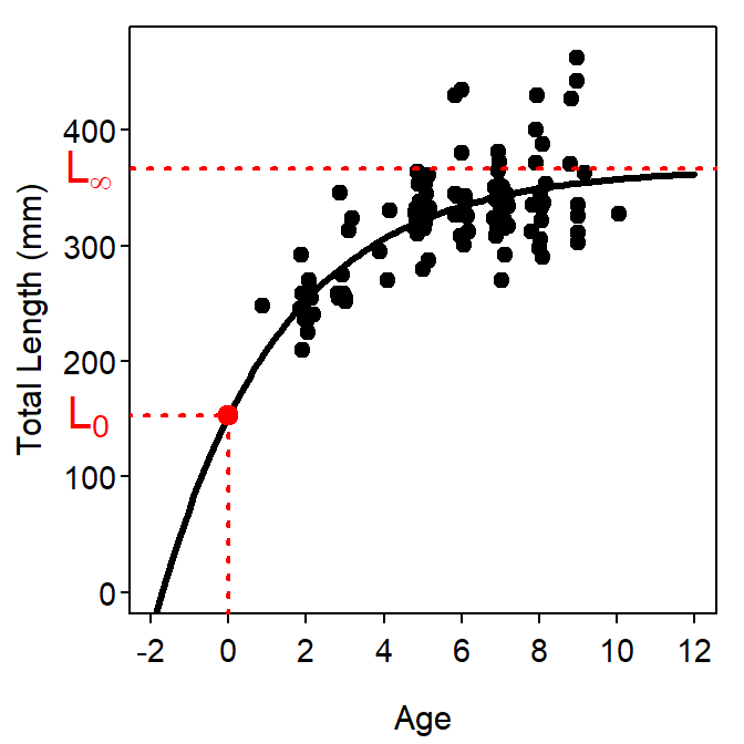
Figure 3: Example of the “original” parameterization of the VBGF fit to size-at-age Atlantic Croaker data. The plot on the left is the fitted model expressed over the observed ages and lengths of the data. The plot on the right is the same fitted model but expressed over a range of ages and lengths that allows for illustrating the meaning of \(L_{\infty}\) and \(L_{0}\).
Gallucci and Quinn (1979) Parameterization
Gallucci and Quinn II (1979) noted that comparisons of “growth” between two groups should involve both \(K\) and \(L_{\infty}\). However, because of the generally high correlation between these two parameters, simultaneous hypothesis tests of these two parameters are compromised and difficult to interpret. To aid comparison between two groups, Gallucci and Quinn II (1979) introduced a new parameter, \(\omega=KL_{\infty}\) which, by solving this quantity for \(L_{\infty}\) and substituting into Equation 1, yields yet another reparameterization of the VBGF,
\[ E[L|t] = \frac{\omega}{K}\left(1-e^{-K(t-t_{0})}\right) \quad \quad \text{(4)} \]
Gallucci and Quinn II (1979) state that \(\omega\) can be thought of as a growth rate because the units are in length-per-time and, in fact, it is representative of the growth rate near \(t_{o}\). Furthermore, they claim that \(\omega\) is the appropriate parameter to use when comparing populations because of its statistical robustness.
Mooij et al. (1999) Parameterization
Mooij et al. (1999) applied the same concept as Gallucci and Quinn II (1979) to Equation 3 rather than Equation 1 to yield the following parameterization,
\[ E[L|t] = L_{\infty}-(L_{\infty}-L_{0})e^{-\frac{\omega}{L_{\infty}}t} \quad \quad \text{(5)} \]
The parameters of this model are interpreted as before with the exception that \(\omega\) is representative of the growth rate near \(L_{0}\).
Schnute Parameterization
All previous parameterizations have two major difficulties – (1) highly correlated parameters and (2) some parameters that are largely extrapolations (the “positions” of \(L_\infty\), \(L_{0}\), and \(t_{0}\) are rarely represented in the data). The VBGF parameterizations shown in this, and the next, section are largely based on “expected values” at known ages and, thus, largely alleviate these difficulties (Ratkowsky 1986). The so-called “Schnute” parameterization (from Quinn II and Deriso (1999)) of the VBGF is,
\[ E[L|t] = L_{1} + (L_{3}-L_{1})\frac{1-e^{-K(t-t_{1})}}{1-e^{-K(t_{3}-t_{1})}} \quad \quad \text{(6)} \]
where \(L_{1}\) is the average length at the youngest age, \(t_{1}\), and \(L_{3}\) is the average length at the oldest age, \(t_{3}\), in the sample.
It is important to note that this parameterization is not more or less parsimonious then any of the previous parameterizations as it still has three parameters – \(L_{1}\), \(L_{3}\), and \(K\) (note that \(t_{1}\) and \(t_{3}\) are constants). However, it does have two major advantages over the previous parameterizations. First, the parameters in this parameterization are less correlated than the parameters in other parameterizations (Gallucci and Quinn II (1979) and see this section) and, thus, more stable. Second, this parameterization is directly comparable to the general growth model developed by Schnute (1981). The major drawback of this parameterization is that comparison to results in the literature or from previous studies is difficult, as the typical parameterization is far more prevalent. Schnute and Fournier (1980) did show, however, that the point estimate of \(L_{\infty}\) and \(t_{0}\) can be obtained from the parameters in the Schnute parameterization as follows,
\[ L_{\infty} = \frac{L_{3}-L_{1}e^{-K(t_{3}-t_{1})}}{1-e^{-K(t_{3}-t_{1})}} \] \[ t_{0} = t_{1} + \frac{1}{K}ln\left(\frac{L_{3}-L_{1}}{L_{3}-L_{1}e^{-K(t_{3}-t_{1})}}\right) \]
A common mistake in the interpretation of the Schnute parameterization is to equate \(L_{2}\) and \(L_{\infty}\). However, \(L_{2} \neq L_{\infty}\) as \(L_{\infty}\) is the average size at the theoretical maximum age and \(L_{2}\) is the average size at the maximum age *in the sample}. Thus, \(L_{2}\leq L_{\infty}\) because the maximum age in the sample is either less than or equal to the theoretical maximum age (Figure 4).
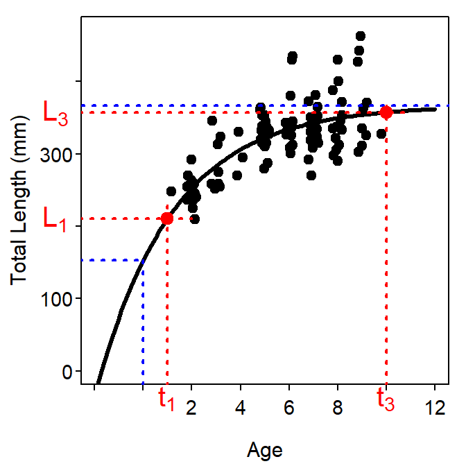
Figure 4: Example of the Schnute parameterization of the VBGF fit to size-at-age Atlantic Croaker data expressed over a range of ages and lengths that allow illustrating the meaning of \(L_{1}\) and \(L_{2}\). In addition, the blue lines correspond to \(L_{\infty}\) from Figure 2 and \(L_{0}\) from Figure 3 for comparative purposes.
Francis (1988) Parameterization
Francis (1988) provided yet another parameterization of the VBGF in his paper comparing the fit of VBGFs to length-at-age data and to tag-recapture data. His basic argument was that the meanings of \(L_{\infty}\) and \(K\) depend on which type of data (and corresponding model) is being fit and that this is an undesirable property. He proposed the following parameterization as a correction to this problem,
\[ E[L|t] = L_{1} + \left(L_{3} - L_{1}\right)\frac{1-r^{2\frac{t-t_{1}}{t_{3}-t_{1}}}}{1-r^2} \quad \quad \text{(8)} \]
where
\[ r = \frac{L_{3}-L_{2}}{L_{2}-L_{1}} \]
where \(L_{1}\), \(L_{2}\), and \(L_{3}\) are the mean lengths at ages \(t_{1}\), \(t_{2}\),and \(t_{3}\), respectivly. The \(t_{1}\) and \(t_{3}\) are arbitrary reference ages (and \(t_{2}\) is half-way between each) but are generally a relatively young (i.e., \(t_{1}\)) and old (i.e., \(t_{3}\)) age. Note that \(r\) is used to simplify the presentation and is not a new parameter. The resultant parameters from this model are effectively the predicted mean lengths-at-age for the three chosen ages (Figure 5).
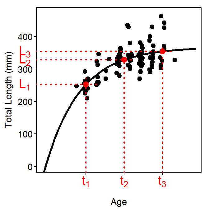
Figure 5: Example of the Francis parameterization of the VBGF fit to size-at-age Atlantic Croaker data expressed over a range of ages and lengths that allow illustrating the meaning of \(L_{1}\), \(L_{2}\), and \(L_{3}\). Note that the arbitrary ages chosen were \(t_{1}\)=2 and \(t_{3}\)=9.
Francis (1988) showed that point estimates of the typical parameters could be derived from these modified parameters as follows,
\[ L_{\infty} = L_{1} + \frac{L_{3}-L_{1}}{1-r^{2}} \] \[ K = \frac{-2log(r)}{t_{3}-t_{1}} \] \[ t_{0} = t_{1} + \frac{1}{K}log\left(\frac{L_{\infty}-L_{1}}{L_{\infty}}\right) \]
Parameterization Comparisons
As noted previously, the different parameterizations of the VBGF are the same model with different parameters (Figure 6). Estimates of parameters that appear in more than one of the parameterizations will be the same among the parameterizations (Table 2). The parameterizations based on expected values (i.e., Schnute and Francis) will generally require fewer iterations to converge when fitting and will result in lower correlations among parameter estimates (Table 2).
Table 2: Parameter estimates and model results from fitting different parameterizations of the VBGF to the male Atlantic Croaker data. Note that \(L_{1}\), \(L_{2}\), and \(L_{3}\) are not comparable between parmaterizations; \(L_{1}\), \(L_{2}\), and \(L_{3}\) correspond to ages 2, 5.5, and 9 in the Francis parameterization; “iters” is the number of iterations to convergence; and \(r_{max}\) and \(r_{mean}\) are the maximum and average absolute value of correlation coefficients among the three parameters.
| Models | \(L_{0}\) | \(L_{\infty}\) | \(K\) | \(t_{0}\) | \(\omega\) | \(L_{1}\) | \(L_{2}\) | \(L_{3}\) | SE | iters | \(r_{max}\) | \(r_{mean}\) |
|---|---|---|---|---|---|---|---|---|---|---|---|---|
| Typical |
|
366 | 0.31 | -1.71 |
|
|
|
|
33 | 4 | 0.97 | 0.93 |
| Original | 153 | 366 | 0.31 |
|
|
|
|
|
33 | 4 | 0.95 | 0.89 |
| Gallucci Quinn |
|
|
0.31 | -1.71 | 115.3 |
|
|
|
33 | 4 | 1.00 | 0.98 |
| Mooij | 153 | 366 |
|
|
115.3 |
|
|
|
33 | 4 | 0.93 | 0.89 |
| Schnute |
|
|
0.31 |
|
|
210 |
|
357 | 33 | 4 | 0.83 | 0.71 |
| Francis |
|
|
|
|
|
253 | 329 | 354 | 33 | 4 | 0.08 | 0.05 |
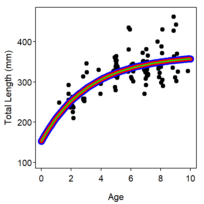
Figure 6: Fits of the typical (blue), Schnute (red), and Francis (green) parameterizations of the VBGF to size-at-age Atlantic Croaker data (auto-generated starting values were used for all parameterizations). Note that the results of all fits are identical and, thus, the fitted lines are directly on top of each other. Different colors and different line widths were used to illustrate this point but may not be readily apparent on the screen or printed page.
Reproducibility Information
- Compiled Date: Wed Dec 29 2021
- Compiled Time: 9:03:07 PM
- R Version: R version 4.1.2 (2021-11-01)
- System: Windows, x86_64-w64-mingw32/x64 (64-bit)
- Base Packages: base, datasets, graphics, grDevices, methods, stats, utils
- Required Packages: FSA, FSAdata, captioner, dplyr, knitr, xtable and their dependencies (car, dunn.test, ellipsis, evaluate, generics, glue, graphics, grDevices, highr, lifecycle, lmtest, magrittr, methods, pillar, plotrix, R6, rlang, sciplot, stats, stringr, tibble, tidyselect, tools, utils, vctrs, withr, xfun, yaml)
- Other Packages: captioner_2.2.3.9000, dplyr_1.0.7, FSA_0.9.1.9000, FSAdata_0.3.8, gdata_2.18.0, knitr_1.36, xtable_1.8-4
- Loaded-Only Packages: assertthat_0.2.1, bslib_0.3.1, compiler_4.1.2, crayon_1.4.2, DBI_1.1.1, digest_0.6.28, ellipsis_0.3.2, evaluate_0.14, fansi_0.5.0, fastmap_1.1.0, generics_0.1.1, glue_1.5.0, gtools_3.9.2, highr_0.9, htmltools_0.5.2, jquerylib_0.1.4, jsonlite_1.7.2, lifecycle_1.0.1, magrittr_2.0.1, pillar_1.6.4, pkgconfig_2.0.3, purrr_0.3.4, R6_2.5.1, rlang_0.4.12, rmarkdown_2.11, sass_0.4.0, stringi_1.7.5, stringr_1.4.0, tibble_3.1.6, tidyselect_1.1.1, tools_4.1.2, utf8_1.2.2, vctrs_0.3.8, xfun_0.28, yaml_2.2.1
- Links: Script / RMarkdown
References
The remainder of this vignette will focus on length data only.↩︎
A weight specific version essentially raises the length-specific version to the power of \(b\), the allometric relation term from the regression of weight on length (i.e., \(W=aL^B\)) – i.e., \(E[W|t] = \left(W_{\infty}\left(1-e^{-K(t-t_{0})}\right)\right)^{b}\).↩︎
Cailliet et al. (2006) notes that \(L_{0}\)=\(L_{\infty}(1-e^{kt_{0}})\).↩︎