Calculate Summary Statistics
Note:
- Make sure to show your work when calculating the standard deviation. The method shown below is one way to show your work that produces consistent results. On assessments, not showing your work will result in a zero for the question.
- Don’t forget to arrange the values from smallest to largest when computing the median. Count the original and your arranged data to make sure you have the same number of values in both.
- The median will be one of the observed values if n is odd, but it will be the average of two observed values if n is even.
- If n is odd such that the median is one of the observed values, then that value is NOT included in either “half” of the data when computing the IQR. In other words, the “lower half” of the data will end right before the median and the “upper half” of the data will end right after the median. See Data Set 2 below.
- Shown below
- Shown above
- Shown below
- Shown above
- Shown below
- Shown above
- Range is 1 to 97.
> sdCalc(c(18,28,25,21,16,24))Demonstration of parts of a std. dev. calculation.
x diffs diffs.sq
1 18 -4 16
2 28 6 36
3 25 3 9
4 21 -1 1
5 16 -6 36
6 24 2 4
sum 132 0 102
Mean = x-bar = 132 / 6 = 22
Variance = s^2 = 102 / 5 = 20.4
Std. Dev = s = sqrt(20.4) = 4.516636> iqrCalc(c(4,54,16,85,52,29,24,71,61,60,2))Median (=52) is the value in position 6.
2 4 16 24 29 [52] 54 60 61 71 85
Q1 (=16) is the value in position 3 of the lower half.
2 4 [16] 24 29
Q3 (=61) is the value in position 3 of the upper half.
54 60 [61] 71 85
**Note that the median (=52) is NOT in both halves.> iqrCalc(c(93,81,34,5,54,84,54,13,1,35,79,63,97,71))Median (=58.5) is the average of values in positions 7 and 8.
1 5 13 34 35 54 [54 63] 71 79 81 84 93 97
Q1 (=34) is the value in position 4 of the lower half.
1 5 13 [34] 35 54 54
Q3 (=81) is the value in position 4 of the upper half.
63 71 79 [81] 84 93 97Histograms I
- An individual is a state.
- The variable is the mean commute time for indivuals 16-years and older in states of the U.S.
- Mean Commute time (mins) is a quantitative, continuous variable.
- 51
- 2
- 25
- 26-28
Frequency and Percentages Tables
Should be performed by hand to match results below
- Frequency Table
- Percentage Table
- Bar Chart
- Shepherds were the most common herding group winners in the Westminster Kennel Club championships winning 28.9% of the time over the last 36 years
group
    Belgian Tervuren Bouvier Des Flandres               Collie                Corgi
                   1                    4                    4                    5
Old English Sheepdog                 Puli             Shepherd    Shetland Sheepdog
5 3 11 5 > percTable(tbl,digits=1)group
Belgian Tervuren Bouvier Des Flandres Collie Corgi
2.6 10.5 10.5 13.2
Old English Sheepdog Puli Shepherd Shetland Sheepdog
13.2 7.9 28.9 13.2 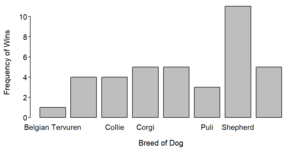
Bar Chart I
- A Northland College student.
- Categorical, nominal.
- Frequency table is below.
- Percentage table is below.
     Love     Money Pregnancy     Other
45 1 0 4 Love Money Pregnancy Other
90 2 0 8