1-Sample t-Test
Recurrence of Cancer Tumors
The tumor recurrence data are loaded and initially examined below. This is a very simple data frame with one variable, months, that contains the number of months until the tumor recurred.
> dfobj <- read.csv("https://raw.githubusercontent.com/droglenc/NCData/master/Tumors.csv")
> str(dfobj)
'data.frame': 42 obs. of 1 variable:
$ months: int 19 18 17 1 21 22 54 46 25 49 ...The 11-steps are shown below along with the R code where appropriate.
- α = 0.10.
- HA: μ > 27 and H0: μ = 27, where μ is the mean months until the tumors recurred.
- Remember to define the parameter.
- A 1-sample t-test will be used because
- one group/population is considered (this group of patients … not comparing two groups),
- a quantitative variable (time to recurrence) was recorded, and
- σ is UNknown (not given in the background).
- These are the three characteristics that separate a 1-sample -test from other tests we will see this semester.
- Please include some sort of description that shows that the characteristics are met and that you are not just listing the characteristics – in other words, include the parts in parentheses.
- If σ is known it will be given in the background information. The standard deviation that will be computed from the data is s.
- This study is observational as the researcher did not create groups or impose a treatment on any individuals. It is not clear or obvious whether the individuals were randomly selected or not.
- This appears to be part of an experiment as the patients were given a placebo. However, there are not groups created by the researchers being compared here so it is not an experiment.
- Do not say that the collection was random if it is not obviously so. Ultimately, this is a problem because the p-value requires randomization. However, we will continue with the analysis in this class, but we will be aware of the potential problems that this poses.
- The assumptions are met because (i) σ is UNknown and (ii) n = 42 ≥ 40.
-
The value of n is seen in the
str()for the data frame shown above the 11 steps. - If the n had been less than 40 then you would need to assess the shape of the histogram.
- Make sure to address whether σ is known or not, even though it feels redundant with Step 3.
Calculations for the next steps are computed with t.test() as demonstrated below.
> t.test(dfobj$months,mu=27,alt="greater",conf.level=0.9)One Sample t-test with dfobj$months
t = 1.8502, df = 41, p-value = 0.03575
alternative hypothesis: true mean is greater than 27
90 percent confidence interval:
28.38127 Inf
sample estimates:
mean of x
31.66667 - x̄ = 31.7.
-
This is from under the “mean of x” output from
t.test().
- t = 1.850 with 41 df.
-
This is from the “t=” output from
t.test().
- p-value=0.036.
-
This is from the “p-value=” output from
t.test().
- Reject H0 because the p-value < α.
- It appears that the mean time for the tumors to reoccur is greater than 27 months.
- Note how the conclusion is about the MEAN time to reoccur and not the time to reoccur. The test is about the summary (i.e., the MEAN) not about individuals.
- Also note the use of “appears” in the summary. This language acknowledges the fact that an error (Type I or Type II) could have been made. No conclusion from a statistical hypothesis test will ever be 100% definitive.
- I am 90% confident that the mean time for the tumors to reoccur is greater than 28.4.
-
This comes from under the “90 percent confidence interval” output from
t.test(). Those results generally show an “interval” but if the first value is replaced with a “-Inf” then the result is an upper bound and if the second value is replaced with a “Inf” (as here) then the result is a lower bound. - This confidence region is a lower bound, so the conclusion is that the mean is greater than the calculated amount.
Note that you will complete all 11 steps when you have the raw data (as we have done here), but you should use t.test() as shown here to perform all of the calculations for you.
2-Sample t-Test
Cholesterol Drug Treatments II
The full 11-steps for this example are in these annotations for the 2-sample t-test class example. However, the calculations required for Steps 5, 6, 7, 8, and 11 may be computed in R if the raw data are available as they were here. Note, however, that the data only had the before and after the drug LDL levels for each patient and not the reduction in LDL. Thus, a reduction in LDL variable had to be computed at shown below. This will not be required for most situations.
> dfobj <- read.csv("https://raw.githubusercontent.com/droglenc/NCData/master/Cholesterol2.csv")
> dfobj$redux <- dfobj$before-dfobj$after
> str(dfobj)
'data.frame': 25 obs. of 4 variables:
$ before: num 2.98 2.7 2.6 2.94 2.55 2.92 2.94 2.94 2.5 3.41 ...
$ after : num 2.63 2.43 2.34 2.41 2.28 2.44 2.45 2.44 2.26 2.96 ...
$ tx : chr "Lipanthyl" "Lipanthyl" "Lipanthyl" "Lipanthyl" ...
$ redux : num 0.35 0.27 0.26 0.53 0.27 ...Another important note is that the data must be “stacked” in order to perform the analyses in R. This means that the data for one group must be stacked below the data for the other group, which will require a variable to explain which group the values correspond to. Fortunately this conforms to our mantra that each row must contain data from only one individual. The first three and last three rows for these data illustrate the stacked format.
> headtail(dfobj) before after tx redux
1 2.98 2.63 Lipanthyl 0.35
2 2.70 2.43 Lipanthyl 0.27
3 2.60 2.34 Lipanthyl 0.26
23 2.62 2.43 Befizal 0.19
24 2.99 2.64 Befizal 0.35
25 2.63 2.45 Befizal 0.18The Levene’s test result is computed with levenesTest() using a formula of the form qvar~cvar, where qvar is the quantitative response variable and cvar is the categorical variable that describes the groups. Of course, the data= argument is also needed. The p-value is shown under the Pr(>F) heading.
> levenesTest(redux~tx,data=dfobj)Levene's Test for Homogeneity of Variance (center = median)
Df F value Pr(>F)
group 1 0.0463 0.8315
23 The histogram of the response variable for each group may be needed for Step 4 (as above) and is easily computed as below (which you have done before). 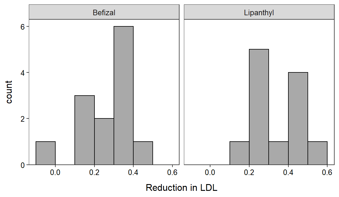
Finally, most of the calculations for Steps 6, 7, 8, and 11 are computed with t.test() using the same formula and data= argument as for levenesTest(). If the variances are found to be equal then you MUST also include var.equal=TRUE. Finally, you should include the null hypothesized value in mu= (will always be zero for 2-sample t-test), the alternative hypothesis sign in alt=, and the confidence level in conf.level= as you have done with the 1-sample t-test.
> t.test(redux~tx,data=dfobj,mu=0,alt="two.sided",conf.level=0.95,var.equal=TRUE) Two Sample t-test with redux by tx
t = -1.4885, df = 23, p-value = 0.1502
alternative hypothesis: true difference in means is not equal to 0
95 percent confidence interval:
-0.18673806 0.03045601
sample estimates:
mean in group Befizal mean in group Lipanthyl
0.2776923 0.3558333 From this output one can see
- The two sample means for Step 6 at the very bottom of the output.
- The t test statistics for Step 7 after “t=”, with the corresponding degrees-of-freedom after “df=”. Note that when you use
t.test()like this you do not need to worry about computing the pooled sample variance or the standard error. - The p-value is after “p-value=” (and, thus, you do not need to use
distrib()). - The confidence region values are under “XX percent confidence interval”. Note that you do not need to find t* nor perform the calculations as they are done here for you. You simply need to write the interpretation.
Note that you will complete all 11 steps when you have the raw data, but you should use t.test() as shown here to perform all of the hard calculations for you.