Urban Runoff

The response variable is IBI.
The explanatory variable is percent impervious surface.
The relationship between IBI and the percent of impervious surface is negative, nonlinear, and moderately strong with no obvious outliers. I did not report the value of the correlation coefficient because of the nonlinear form.

R Code and Results

> d <- read.csv("IBI.csv")

> ggplot(data=d,mapping=aes(x=imp,y=IBI)) +
    geom_point(pch=21,color="black",fill="lightgray") +
    labs(x="Percent Impervious Land",y="Benthic Index of Biotic Integrity") +
    theme_NCStats()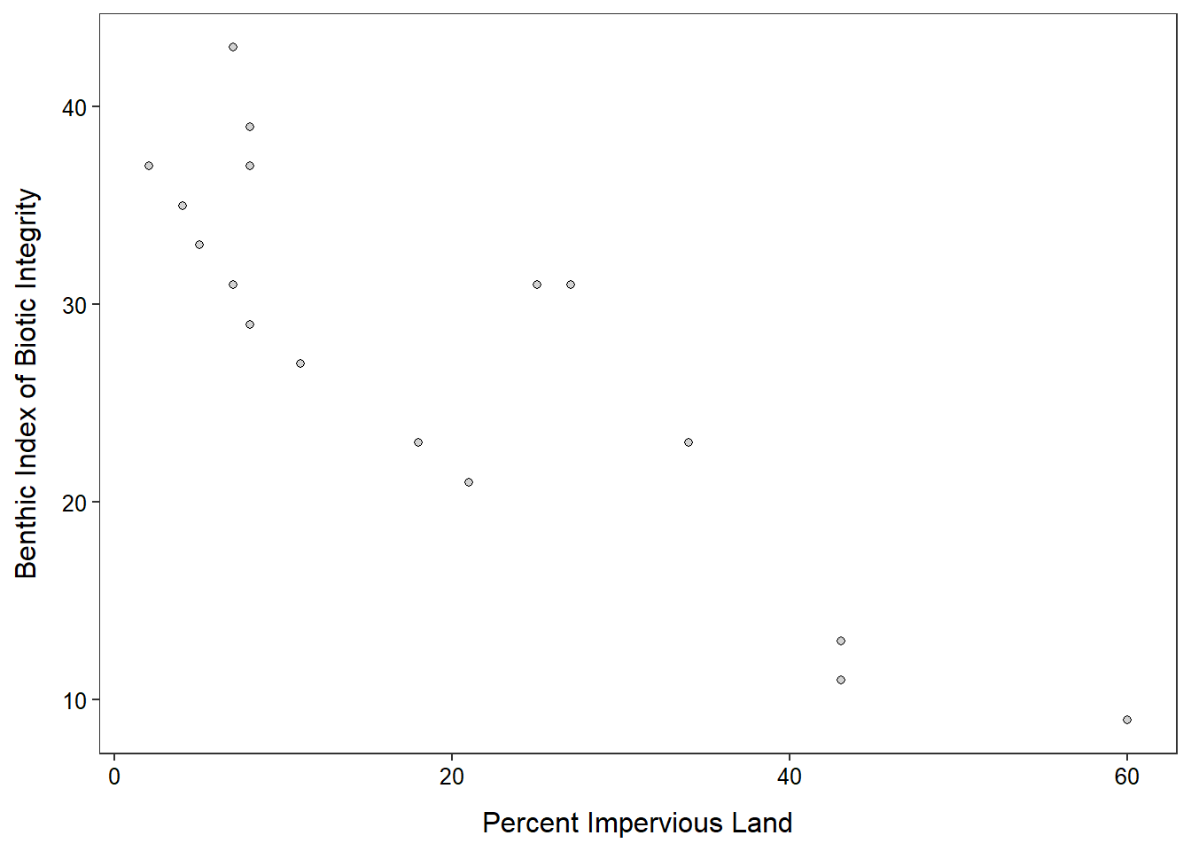

Lights and Nearsightedness

The percentage of children that slept with a “night light” that did not develop nearsightedness is 65.9% (see row percent table).
The percentage of all children that slept with a “lamp” and developed nearsightedness is 8.6% (see total percent table).
The percentage of children that slept in “no light” conditions that then developed nearsightedness is 9.9% (see row percent table).
A total of 17 children slept in “no light” conditions and developed nearsightedness (see frequency table).
The percentage of children that developed nearsightedness is 28.6% (see total percent table).
The percentage of children that developed nearsightedness that slept with a “lamp” is 29.9% (see column percent table).
It appears that the percentage of children that developed nearsightedness is greater when the child slept with some sort of light (either a lamp or a night light), with a somewhat greater prevalence of nearsightedness with the lamp (see row percent table).

R Code and Results

> d <- read.csv("Nearsight.csv")

> tbl <- xtabs(~Light+Nearsightedness,data=d)
> addmargins(tbl)

             Nearsightedness
Light          No Yes Sum
  lamp         34  41  75
  night light 153  79 232
  no light    155  17 172
  Sum         342 137 479

> ( row.tbl <- percTable(tbl,margin=1) )

             Nearsightedness
Light            No   Yes   Sum
  lamp         45.3  54.7 100.0
  night light  65.9  34.1 100.0
  no light     90.1   9.9 100.0

> ( col.tbl <- percTable(tbl,margin=2) )

             Nearsightedness
Light            No   Yes
  lamp          9.9  29.9
  night light  44.7  57.7
  no light     45.3  12.4
  Sum          99.9 100.0

> ( perc.tbl <- percTable(tbl) )

             Nearsightedness
Light            No   Yes   Sum
  lamp          7.1   8.6  15.7
  night light  31.9  16.5  48.4
  no light     32.4   3.5  35.9
  Sum          71.4  28.6 100.0

Wolves and Whitetail Deer

The relationship between the territory size of wolf pakces and the abundance of deer is linear, negative, moderately strong (r=-0.787), and without any obvious outliers. I assessed the strength of the relationship with the correlation coefficient (r) because the form is linear and there are no outliers. [Note that I can see an argument for calling this nonlinear; if so, make sure you don’t use r to assess strength.]

R Code and Results

> d <- read.csv("Wolves2.csv")

> ggplot(data=d,mapping=aes(x=deer,y=terr)) +
    geom_point(pch=21,color="black",fill="lightgray") +
    labs(x="Abundance of Deer (#/km^2)",y="Wolf Territory Size (km^2)") +
    theme_NCStats()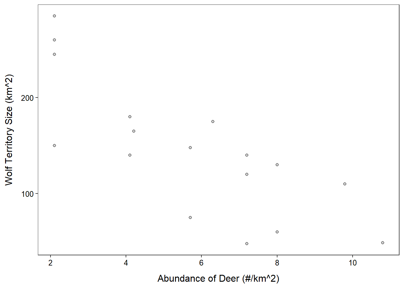

> corr(~deer+terr,data=d,digits=3)

[1] -0.787