Mortality is a key component to understanding the population dynamics of fish species. Total mortality is often estimated from the sequential decline observed in cohorts of fish. The catch curve regression and Chapman-Robson methods used to analyze this decline are collectively called catch-curve methods and form the topic of these notes.
Data Requirements
In a population that is closed to emigration or immigration, the annual mortality rate (\(A\)) between two times is equal to the number of deaths during the time period divided by the population size at the start of the time period, or
\[ A = \frac{N_{t}-N_{t+1}}{N_{t}} = 1-\frac{N_{t+1}}{N_{t}} \]
Unfortunately, it is usually not possible to know the number of fish in a population. However, if the catch of fish (\(C\)) is proportional to the size of the population, i.e., \(C_{t}=vN_{t}\), then algebra quickly shows that
\[ A = \frac{C_{t}-C_{t+1}}{C_{t}} = 1-\frac{C_{t+1}}{C_{t}} \]
Thus, the mortality of a cohort of fish can be estimated from knowing the catches of fish at various times. In many fisheries, fisheries scientists “record time” by estimating the age of fish. Thus, the number of fish captured at varous ages, i.e., catch-at-age data, can be used to estimate mortality rates of fish populations.
In the statistical literature, longitudinal data is data that occurs when multiple samples are taken from the same group of individuals over time. The catches of fish from the same cohort over time is an example of longitudinal data. Longitudinal fisheries data takes many years to collect, which can be very costly and impart a long time-lag in management decisions.
Catch data from a single year across many cohorts of fish will be identical to longitudinal data of a single cohort if each cohort sampled began with the same number of fish (i.e., recruitment is constant) and if the mortality rate is constant across all ages and years. For example, the catches-at-age of the hypothetical 2002 and 2006 cohorts is shown on diagonals in Table 1 and are equal to the catch-at-age for fish in the 2009 capture year. The catch in a single year is called cross-sectional data because it “crosses” several cohorts of fish.
Table 1: The hypothetical catch of fish by age and capture year. The longitudinal catch of the 2002 and the partial 2006 year-classes of fish are shown by the two sets of diagonal cells highlighted in dark grey. The cross-sectional catch in the 2009 capture year is shown by the column of cells highlighted in light grey. All data were modeled with Equation 2 assuming that \(N_{0}=500\), \(Z=-log(0.7)\), and \(v=0.1\).
| Capture Year | ||||||||||||
|---|---|---|---|---|---|---|---|---|---|---|---|---|
| Age | 2002 | 2003 | 2004 | 2005 | 2006 | 2007 | 2008 | 2009 | 2010 | 2011 | 2012 | 2013 |
| 0 | 50.0 | 50.0 | 50.0 | 50.0 | 50.0 | 50.0 | 50.0 | 50.0 | 50.0 | 50.0 | 50.0 | 50.0 |
| 1 | 35.0 | 35.0 | 35.0 | 35.0 | 35.0 | 35.0 | 35.0 | 35.0 | 35.0 | 35.0 | 35.0 | 35.0 |
| 2 | 24.5 | 24.5 | 24.5 | 24.5 | 24.5 | 24.5 | 24.5 | 24.5 | 24.5 | 24.5 | 24.5 | 24.5 |
| 3 | 17.1 | 17.1 | 17.1 | 17.1 | 17.1 | 17.1 | 17.1 | 17.1 | 17.1 | 17.1 | 17.1 | 17.1 |
| 4 | 12.0 | 12.0 | 12.0 | 12.0 | 12.0 | 12.0 | 12.0 | 12.0 | 12.0 | 12.0 | 12.0 | 12.0 |
| 5 | 8.4 | 8.4 | 8.4 | 8.4 | 8.4 | 8.4 | 8.4 | 8.4 | 8.4 | 8.4 | 8.4 | 8.4 |
| 6 | 5.9 | 5.9 | 5.9 | 5.9 | 5.9 | 5.9 | 5.9 | 5.9 | 5.9 | 5.9 | 5.9 | 5.9 |
| 7 | 4.1 | 4.1 | 4.1 | 4.1 | 4.1 | 4.1 | 4.1 | 4.1 | 4.1 | 4.1 | 4.1 | 4.1 |
| 8 | 2.9 | 2.9 | 2.9 | 2.9 | 2.9 | 2.9 | 2.9 | 2.9 | 2.9 | 2.9 | 2.9 | 2.9 |
| 9 | 2.0 | 2.0 | 2.0 | 2.0 | 2.0 | 2.0 | 2.0 | 2.0 | 2.0 | 2.0 | 2.0 | 2.0 |
| 10 | 1.4 | 1.4 | 1.4 | 1.4 | 1.4 | 1.4 | 1.4 | 1.4 | 1.4 | 1.4 | 1.4 | 1.4 |
Catch Curve Regression Methods
Annual mortality can be estimated from catch data for two ages as shown above. However, fisheries scientists prefer estimates that are more synthetic, i.e., based on more ages. The two most common methods for computing synthetic estimates of mortality rates are the catch-curve regression and Chapman-Robson methods. The regression method is discussed in this section.
Regression Model
The decline in individuals with age can be theoretically modeled with a modified continuous exponential population model. Because the population is closed with the exception of mortality, the instantaneous population growth rate parameter in the exponential population model is replaced with an instantaneous total mortality parameter (\(Z\)). Thus, the modified model is
\[ N_{t} = N_{0}e^{-Zt} \quad \quad \text{(1)} \]
where \(N_{t}\) is the population size at time \(t\) and \(N_{0}\) is the initial population size.
The catch of fish at age \(t\) is proportional to the number of fish of age \(t\), or \(C_{t}=vN_{t}\), as mentioned previously.1 This is rearranged to show that the relationship between population size and catch is \(N_{t}=\frac{C_{t}}{v}\) and substituted into Equation 1 to reveal
\[ \frac{C_{t}}{v} = N_{0}e^{-Zt} \quad \quad \text{ } \] \[ C_{t} = vN_{0}e^{-Zt} \quad \quad \text{(2)} \]
In contrast to Equation 1 the variables in Equation 2 (catch-at-age, \(C_{t}\), and age, \(t\)) are directly observable. The shape of Equation 2 (Figure 1-Left) follows the expected exponential decline. As is typical with exponential models, natural logarithms of both sides of Equation 2 yields
\[ log(C_{t}) = log(vN_{0})-Zt \quad \quad \text{(3)} \]
which is in the form of a linear equation with \(log(C_{t})\) on the y-axis and \(t\) on the x-axis (Figure 1-Right). Of great interest in Equation 3 is that the negative of the slope is \(Z\). Thus, the negative of the slope of the linear regression between \(log(C_{t})\) and \(t\) is an integrative measure of the instantaneous total mortality rate experienced by this cohort of fish over time.


Figure 1: Ideal plots of catch versus age (Left) and the natural log of catch versus age (Right) for a single cohort of fish. The right graph is called a longitudinal catch curve. The change in \(log(C_{t})\) for a unit change in \(t\) is emphasized on the catch curve to reinforce the idea that the slope of the idealized catch curve is \(Z\).
Equation 1 can also be recast by assuming that catch-at-age (\(C_{t}\)) is proportional to the number-at-age and the amount of effort expended to catch those fish (i.e., \(E_{t}\)). Thus, \(C_{t}=qE_{t}N_{t}\), where \(q\) represents a constant proportion of the population captured by one unit of effort. This model can be rearranged to show that the relationship between population size and catch-per-unit-effort is \(N_{t}=\frac{1}{q}\frac{C_{t}}{E_{t}}\). This is substituted into Equation 1 and simplified to reveal
\[ \frac{1}{q}\frac{C_{t}}{E_{t}} = N_{0}e^{-Zt} \quad \quad \quad \quad \text{ } \]
\[ \frac{C_{t}}{E_{t}} = qN_{0}e^{-Zt} \quad \quad \text{(4)} \]
Again, the variables in Equation 4 (catch-per-unit-effort, \(\frac{C_{t}}{E_{t}}\), and age, \(t\)) are directly observable. Furthermore, natural logarithms of both sides of Equation 4 yields
\[ log(\frac{C_{t}}{E_{t}}) = log(qN_{0})-Zt \quad \quad \text{(5)} \]
which again is in the form of a linear equation with \(log(\frac{C_{t}}{E_{t}})\) on the y-axis and \(t\) on the x-axis. Thus, the negative of the slope of the regression between \(log(\frac{C_{t}}{E_{t}})\) and \(t\) is also an integrative measure of the instantaneous total mortality rate experienced by this cohort of fish over time. In other words, the y-axis variable can be either catch or catch-per-unit-effort data. The specifics of this regression methodology are discussed in Ogle (2016).
Characteristics
All catch curves have three regions of interest: an ascending left limb, a domed middle portion, and a descending right limb (Figure 2). The ascending left limb represents age-classes of fish that are not yet fully vulnerable to the gear used in the fishery. Fish in these age-classes are said to have “not fully recruited to the fishery.” The catches of fish in these age-classes are not useful for estimating the total mortality rate.
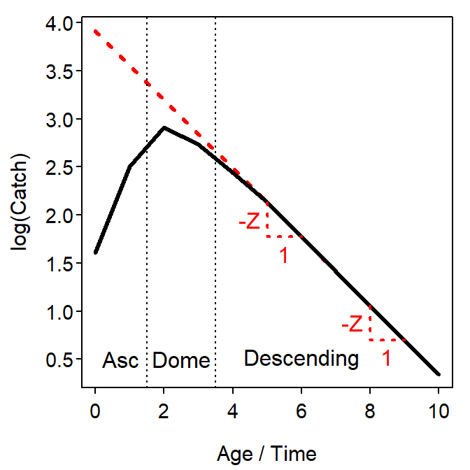
Figure 2: Idealized catch curve (plot of the natural log of catch versus age) illustrating the ascending, domed, and descending portions. The red dotted line represents the idealized catch curve if all age-classes were fully recruited to the fishery.
The domed portion of the catch-curve generally consists of age-classes of fish that are nearly, but not completely, recruited to the fishery. The relative width of the domed portion provides some insight into the rate of recruitment. For example, a very sharply pointed dome indicates that the fish recruit rather “quickly.”2 In contrast, a relatively rounded dome shows that fish recruit to the exploited phase of the population more slowly, perhaps requiring several years before the mean size of fish in that year-class is sufficiently large to ensure capture upon encounter with the gear. Fish in age-classes in the domed portion of the catch curve are also excluded from use when estimating \(Z\). Despite the exclusion of age-classes in the ascending limb and domed portion of the catch curve it is, however, imperative to have some animals from these age-classes in your sample, so that you can identify the important descending limb of the catch curve.
The descending left limb of the catch curve represents the regular decline of fully-recruited individuals in the fishery. Thus, \(Z\) can be estimated by applying the concept of Equation 3 to the catches of fish in the ages corresponding only to the descending portion of the catch curve. There is some debate about how the descending limb is defined in practice. Additionally, the portion of the descending limb corresponding to the older ages is often poorly represented in the catch data because these individuals are relatively rare. At times, some catch data for older ages may be ignored.
Smith et al. (2012) suggested that a weighted regression (discussed in Ogle (2016)) with all age-classes older than and including the age with the maximum catch should be used.
Instantaneous vs. Annual Mortality Rates
The instantaneous mortality rate (\(Z\)) that is estimated via the catch curve method is a measure of (i) how much the natural log of number of individuals declines annually or (ii) how much the actual number of individuals declines in an imperceptibly short period of time (i.e., in an “instant”). The instantaneous mortality rate has some very useful mathematical properties, but providing a practical interpretation of its meaning is difficult – e.g., what does it mean if the log number of individuals declines by 0.693 or if the population changes by 0.693 in a “millisecond” of time? Fortunately, the instantanous mortality rate can be easily converted to an annual mortality rate (\(A\)), the proportion of the population that suffers mortality in a given year, with
\[ A = 1-e^{-Z} \]
Thus, a \(Z\) of 0.693 corresponds to an \(A\) of \(1-e^{-0.693}\) or 0.500. Thus, this largely uninterpretable value of \(Z\) corresponds to an annual mortality rate of 50.0%. In other words, an average of 50.0% of the population dies on an annual basis.
Reproducibility Information
- Compiled Date: Wed Dec 29 2021
- Compiled Time: 8:38:32 PM
- R Version: R version 4.1.2 (2021-11-01)
- System: Windows, x86_64-w64-mingw32/x64 (64-bit)
- Base Packages: base, datasets, graphics, grDevices, methods, stats, utils
- Required Packages: FSA, captioner, knitr and their dependencies (car, dplyr, dunn.test, evaluate, graphics, grDevices, highr, lmtest, methods, plotrix, sciplot, stats, stringr, tools, utils, withr, xfun, yaml)
- Other Packages: captioner_2.2.3.9000, FSA_0.9.1.9000, knitr_1.36
- Loaded-Only Packages: bslib_0.3.1, compiler_4.1.2, digest_0.6.28, evaluate_0.14, fastmap_1.1.0, highr_0.9, htmltools_0.5.2, jquerylib_0.1.4, jsonlite_1.7.2, magrittr_2.0.1, R6_2.5.1, rlang_0.4.12, rmarkdown_2.11, sass_0.4.0, stringi_1.7.5, stringr_1.4.0, tools_4.1.2, xfun_0.28, yaml_2.2.1
- Links: Script / RMarkdown