R Appendix
library(FSA)
library(tidyverse)
library(ggplot2)

yp <- read.csv("https://raw.githubusercontent.com/droglenc/FSAdata/master/data-raw/YPerchSB1.csv") %>%
  mutate(lcat10=lencat(tl,w=1),
         gcat=psdAdd(tl,species="Yellow Perch",unit="cm"))
str(yp)
'data.frame':   2074 obs. of  4 variables:
 $ tl    : num  7.4 5.4 6.7 6 7.5 6.6 6.8 6.1 6.1 7.4 ...
 $ loc   : chr  "inner" "inner" "inner" "inner" ...
 $ lcat10: num  7 5 6 6 7 6 6 6 6 7 ...
 $ gcat  : Factor w/ 6 levels "substock","stock",..: 1 1 1 1 1 1 1 1 1 1 ...
ypin <- filter(yp,loc=="inner")
ypout <- filter(yp,loc=="outer")

freq <- xtabs(~loc+lcat10,data=yp)
freq
       lcat10
loc       5   6   7   8   9  10  11  12  13  14  15  16  17  18  19  20  21  22  23  24
  inner   9  15  13   6  12  66  80  94 130 131 113 136 112  92  89  34  31  19   6  11
  outer   3   3  11  27  15  29  37  28  23  13  67  69  89  94 109  43  43  30  26  25
       lcat10
loc      25  26  27  28  29
  inner   5   3   3   0   0
  outer  23  20  17  11   9
psdin <- psdCalc(~tl,data=ypin,species="Yellow Perch",
what="traditional",units="cm")
psdout <- psdCalc(~tl,data=ypout,species="Yellow Perch",
what="traditional",units="cm")
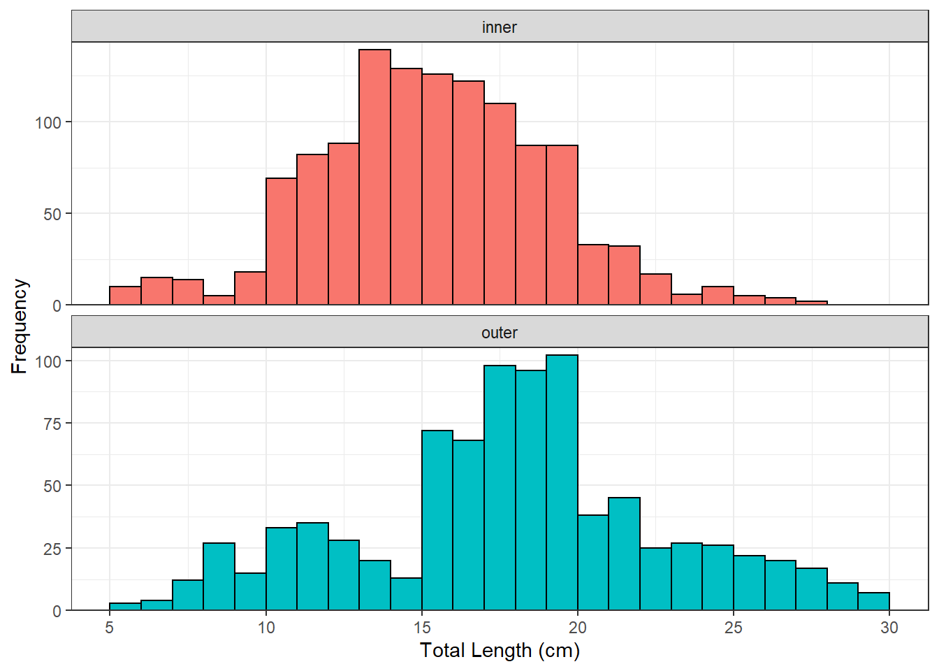
ggplot(data=yp,mapping=aes(x=tl,fill=loc)) +
geom_histogram(binwidth=1,boundary=0,color="black") +
scale_x_continuous(name="Total Length (cm)",breaks=seq(5,30,5)) +
scale_y_continuous(name="Frequency",expand=expansion(mult=c(0,0.03))) +
theme_bw() +
theme(legend.position="none") +
facet_wrap(vars(loc),scale="free_y",ncol=1)