R Appendix
library(FSA)
library(tidyverse)
library(patchwork)

df <- read.csv("https://raw.githubusercontent.com/droglenc/FSAdata/master/data-raw/InchLake2.csv")
wsVal("Bluegill")
    species  units   type ref measure method min.TL    int slope         source
26 Bluegill metric linear  75      TL  Other     80 -5.374 3.316 Hillman (1982)
bg <- df %>%
  filter(species=="Bluegill") %>%
  mutate(length=length*25.4,
         ws=10^(-5.374+3.316*log10(length)),
         wr=weight/ws*100,
         gcat=psdAdd(length,species="Bluegill")) %>%
  filter(length>=80)

bg07 <- bg %>% filter(year==2007)
bg08 <- bg %>% filter(year==2008)
Summarize(wr~gcat,data=bg07,digits=1)
       gcat  n mean   sd  min   Q1 median   Q3   max
1     stock 24 80.0 18.8 45.8 68.5   84.8 92.5 116.2
2   quality 38 89.8  7.5 71.2 85.0   90.9 95.3 101.6
3 preferred 21 96.3  5.0 88.3 92.0   97.3 99.7 103.4
aov07 <- lm(wr~gcat,data=bg07)
anova(aov07)
Analysis of Variance Table

Response: wr
          Df Sum Sq Mean Sq F value    Pr(>F)
gcat       2   3064 1532.00  11.425 4.319e-05
Residuals 80  10727  134.09
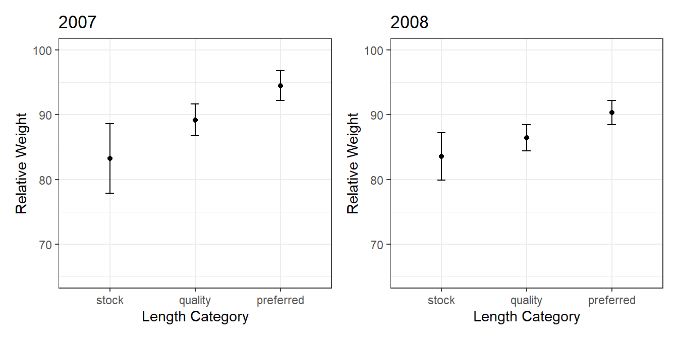
g07 <- ggplot(data=bg07,mapping=aes(x=gcat,y=wr)) +
  stat_summary(fun=mean,geom="point") +
  stat_summary(fun.data=mean_cl_normal,geom="errorbar",width=0.1) +
  scale_x_discrete(name="Length Category") +
  scale_y_continuous(name="Relative Weight",limits=c(65,100)) +
  theme_bw() +
  labs(title="2007")
Summarize(wr~gcat,data=bg08,digits=1)
       gcat  n mean   sd  min   Q1 median   Q3  max
1     stock 24 72.7 16.8 43.5 55.1   78.2 86.0 96.8
2   quality 28 86.4  5.3 78.6 82.7   86.0 89.9 99.7
3 preferred 25 90.4  4.5 82.0 87.8   90.3 94.0 98.3
aov08 <- lm(wr~gcat,data=bg08)
anova(aov08)
Analysis of Variance Table

Response: wr
          Df Sum Sq Mean Sq F value    Pr(>F)
gcat       2 4223.8 2111.91  20.135 1.043e-07
Residuals 74 7761.7  104.89
g08 <- ggplot(data=bg08,mapping=aes(x=gcat,y=wr)) +
  stat_summary(fun=mean,geom="point") +
  stat_summary(fun.data=mean_cl_normal,geom="errorbar",width=0.1) +
  scale_x_discrete(name="Length Category") +
  scale_y_continuous(name="Relative Weight",limits=c(65,100)) +
  theme_bw() +
  labs(title="2008")
g07 + g08