Lake Ontario Rock Bass

  1. There are 135 fish that were aged and 1153 fish that were not aged.
  2. Answers are below.
    1. There were 10 fish in the 180-mm category in the aged sample.
    2. There were 24 age-7 fish in the aged sample.
    3. The proportion of fish in the 140-mm TL category that were age-4 was 0.9.
    4. The proportion of fish in the 200-mm TL category that were age-8 was 0.1.
  3. Answers are below
    1. The proportion of fish in the 210-mm TL category that should be assigned age-5 was 0.1.
    2. Of 30 Rock Bass in the 180-mm TL category, 12 should be assigned age-5.
    3. This age-length key is pretty “clean.” There are some anomolies with age-8 and age-9 fish near 200 mm and age-11 fish from 230 to 270 mm, but these proportions are fairly small.
  4. Answers are below
    1. There were 263 age-5 fish after applying the age-length key.
    2. There were 6 age-11 fish after applying the age-length key.
    3. The age distribution is shown in the second plot below.
    4. There were 43 total fish in the 150-mm TL category.
    5. The mean TL of age-5 fish is 187.5 mm.
    6. The length-at-age plot is shown in the third plot below.

R Appendix

library(FSA)
library(tidyverse)
library(ggplot2)

rb <- read.csv("https://raw.githubusercontent.com/droglenc/FSAdata/master/data-raw/RockBassLO2.csv") %>%
  mutate(lcat10=lencat(tl,w=10,as.fact=TRUE))
rba <- filter(rb,!is.na(age))
rbl <- filter(rb,is.na(age))

## Summary tables for aged sample
xtabs(~lcat10,data=rba)
xtabs(~age,data=rba)
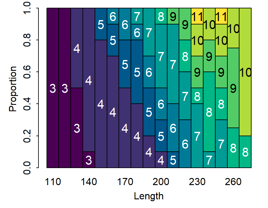
## Make ALK
agelendist <- xtabs(~lcat10+age,data=rba)
alk <- prop.table(agelendist ,margin=1)
alkPlot(alk)

## Apply the ALK
rblmod <- alkIndivAge(alk,age~tl,data=rbl)
headtail(rbl)
headtail(rblmod)

## Combine two dfs with ages and compute some summaries
rbamod <- rbind(rba,rblmod)

(agedist <- xtabs(~age,data=rbamod))

(lendist <- xtabs(~lcat10,data=rbamod))

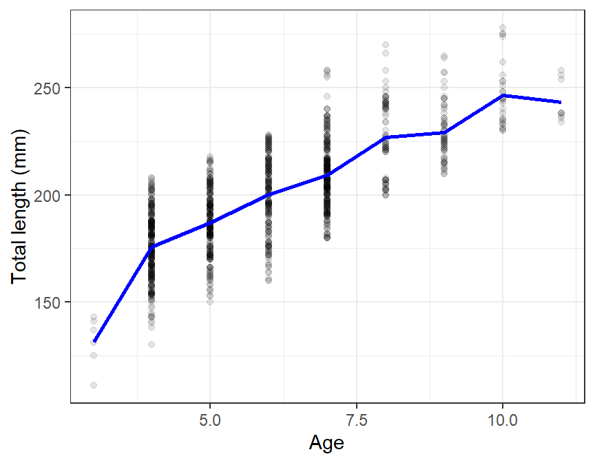
lenatage <- rbamod %>%
  group_by(age) %>%
  summarize(n=n(),
            mntl=mean(tl),
            sdtl=sd(tl))
lenatage

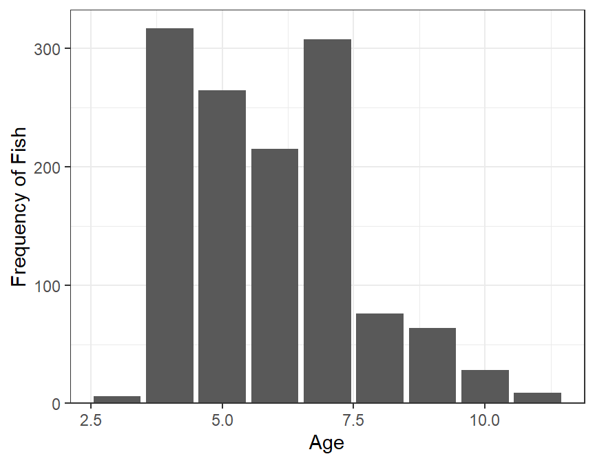
ggplot(data=rbamod,mapping=aes(x=age)) +
  geom_bar() +
  scale_x_continuous(name="Age") +
  scale_y_continuous(name="Frequency of Fish",expand=expansion(c(0,0.05))) +
  theme_bw()

ggplot() +
  geom_point(data=rbamod,mapping=aes(x=age,y=tl),color=col2rgbt("black",1/10)) +
  geom_line(data=lenatage,mapping=aes(x=age,y=mntl),color="blue",size=1) +
  scale_x_continuous(name="Age") +
  scale_y_continuous(name="Total length (mm)") +
  theme_bw()